Dimension Reduction and LASSO using Pointwise and Group Norms

(1)

Worcester Polytechnic Institute

Digital WPI

Masters Theses (All Theses, All Years)

Electronic Theses and Dissertations

2018-12-11

Dimension Reduction and LASSO using

Pointwise and Group Norms

Melanie A. Jutras

Worcester Polytechnic Institute

Follow this and additional works at:

https://digitalcommons.wpi.edu/etd-theses

This thesis is brought to you for free and open access byDigital WPI. It has been accepted for inclusion in Masters Theses (All Theses, All Years) by an

Repository Citation

Jutras, Melanie A., "Dimension Reduction and LASSO using Pointwise and Group Norms" (2018).Masters Theses (All Theses, All Years).

1254.

(2)

WORCESTER POLYTECHNIC INSTITUTE

Dimension Reduction and LASSO

using

Pointwise and Group Norms

by Melanie Jutras

A thesis

Submitted to the Faculty of

WORCESTER POLYTECHNIC INSTITUTE in partial fulfillment of the requirements for the

Degree of Master of Science in

Data Science

December 2018

APPROVED:

Professor Randy C. Paffenroth, Advisor:

(3)

Abstract

Data Science Master of Science by Melanie Jutras

Principal Components Analysis (PCA) is a statistical procedure commonly used for the purpose of analyzing high dimensional data. It is often used for dimen-sionality reduction, which is accomplished by determining orthogonal compo-nents that contribute most to the underlying variance of the data. While PCA is widely used for identifying patterns and capturing variability of data in lower dimensions, it has some known limitations. In particular, PCA represents its results as linear combinations of data attributes. PCA is therefore, often seen as difficult to interpret and because of the underlying optimization problem that is being solved it is not robust to outliers. In this thesis, we examine extensions to PCA that address these limitations. Specific techniques researched in this thesis include variations of Robust and Sparse PCA as well as novel combinations of these two methods which result in a structured low-rank approximation that is robust to outliers. Our work is inspired by the well known machine learning methods of Least Absolute Shrinkage and Selection Operator (LASSO) as well as pointwise and group matrix norms. Practical applications including robust and non-linear methods for anomaly detection in Domain Name System network data as well as interpretable feature selection with respect to a website classifi-cation problem are discussed along with implementation details and techniques for analysis of regularization parameters.

(6)

Executive Summary

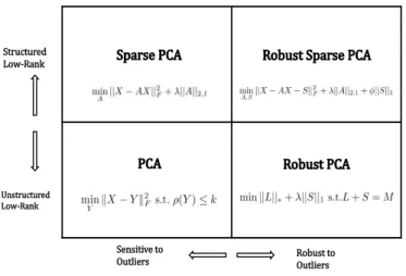
This thesis examines novel methods for robust and low-rank transformations of high dimensional data. Specifically, we will demonstrate two distinct approaches to develop mathematical models based on underlying patterns and structure. The focus of one approach is to detect anomalies in high dimensional data by separating the original data into a low rank component of normal data and a sparse component which contains gross outliers. This type of processing is easily visualized in terms of images or video. One can imagine separating an image in two - one part containing the subject of the image and another which simply contains anomalies or corruptions that may have been present in the original data. A second approach to dimensionality reduction explored in this research involves a similar separation of high dimensional data into low-rank and sparse components, however, with more structured and interpretable results. An example which illustrates the necessity of such an approach is that of gene expression data. Data containing many more features than samples, sometimes millions of features per sample, must be reduced in an interpretable fashion. Of course, as with all real data, corruptions and outliers exist, and so it is useful to be able to provide robust solutions. Although the methods we explore here are applicable to many different types of high dimensional data, we are not focused on image data or gene expression data. The application of the research methods described here will be demonstrated on two very different sets of computer network data in the interest of contributing to the important domain of cybersecurity. The quadrant view in Figure 1 illustrates various methods of PCA explored in this thesis.

Unstructured Low-Rank Structured Low-Rank Robust to Outliers Sensitive to Outliers

(7)

We begin with an overview of the widely used Principal Components Analy-sis (PCA) method of dimensionality reduction. We precisely define the underly-ing mathematics with a particular focus on a least-squares view of the method. After presenting various mathematical background necessary for the remainder of the work, additional variants of PCA are defined and explored. A known limitation of PCA is its sensitivity to outliers. A variant of PCA which is ro-bust to outliers, Roro-bust Principal Components Analysis (RPCA) is presented in Section 3.5.1. The benefits of Robust PCA are described including its use of two important pointwise matrix norms, the nuclear norm and the `1 norm. These

norms are defined in Section 3.4.2. Our experiments reveal how the method is useful for separating high dimensional DNS data into low-rank and sparse com-ponents. In a novel discovery regarding the DNS data, Kernel PCA is utilized as well providing remarkable results.

Next, we move on to dimensionality reduction with a structured sparsity re-sulting from Sparse PCA methods which are described in Section 3.25. This structured sparsity is made possible by the group `2,1 norm also described in

Section 3.4.2. Finally, a variant of PCA which combines the benefits of struc-tured low-rank and robustness will be presented in a novel formulation of Robust Sparse PCA.

min

A,S||X−AX−S|| 2

F+λ||A||2,1+φ||S||1 (1)

The parameters λ and φ in this optimization problem require careful tuning to provide desired results. A unique scoring method combined with three di-mensional data visualization was constructed for the purpose of analyzing our Robust Sparse PCA formulation.

The details of the formulation are revealed in section 3.5.2. We apply these methods to a dataset containing malicious and benign websites and demonstrate the benefits of reducing dimensionality by uncovering low-rank data with sparse features, which also has outliers removed.

(8)

Acknowledgments

This research was performed in partial fulfillment of a Master of Data Science degree at Worcester Polytechnic Institute. The Data Science Masters Thesis is interdisciplinary in nature combining Data Science, Mathematics and Computer Science. That being said, there were professors from all disciplines who inspired me and taught me various elements that contributed to my work. First and foremost, I extend my sincerest gratitude to my advisor and favorite professor, Dr. Randy Paffenroth. Brilliant yet approachable and always generous with time and thought-provoking discussion.

I am inspired by my peers in the research group who provided insightful and detailed accounts of their ongoing research each week. Special thanks go out to Chong Zhou who was always willing to help not only me (his assigned mentee), but others as well. I sincerely appreciate the thorough reading and helpful comments of my thesis reader, Dr. Lane Harrison. I also owe many thanks to the bonus mentor and employer I acquired through this process, Dr. Les Servi and The MITRE Corporation for the generous contribution of real-world data as well as endless hours of mathematical discussion, guidance and support in this endeavor.

Finally, none of this would be possible without the support of my family who are my biggest fans.

(9)

Chapter 1 Introduction

We live in a world of high dimensional data. Data collection and storage solu-tions have enabled us to have access to seemingly unlimited supplies of infor-mation. The human brain cannot even imagine, let alone visualize, the high dimensions. This thesis is about dimensionality reduction and the search for underlying structure. Pattern and structure can not always be determined with traditional statistical methods due to the curse of dimensionality and the general increased complexity involved with today’s data. There is a need for unsuper-vised mathematically based methods for finding patterns in data. Principal Components Analysis (PCA) is one of the most commonly used techniques in machine learning for the purpose of gaining insight with respect to explained variance. Although it is widely used and provides a great deal of information, it is limited in the sense that it is not highly interpretable and it is not robust to outliers.

We describe in this work, our research contributions in this area to the need for anomaly detection in sparse high dimensional computer network traffic, specifi-cally DNS data. We also explore the need for minimizing the number of measures required for classification of various data. Again, due to the nature of the data we are able to obtain, traditional methods for selecting a sparse set of features has become too complex to achieve. We demonstrate solutions for this type of problem with a focus on finding sparse measures related to classifying malicious and benign websites.

Our approaches for dimensionality reduction provide solutions robust to outliers by extending PCA in terms of the least squares methods of the Eckart-Young theorem. Our method takes advantage of pointwise and group norms which transform the data, providing a result that is interpretable and is both low-rank and sparse in the features.

(10)

1.1 Previous Work

Previous work in this area can be attributed dating back to the early 1800s with development of the theory behind the singular value decomposition (SVD) [12], research in the early 1900s with PCA followed in 1936 by the Eckart-Young theorem. [11]. More recent advances and work that are more directly applicable to the foundation of this thesis include Robust PCA by Candes et al. [1], expanded by Paffenroth et al. [2], as well as the Elastic-Net [19] and various Sparse PCA formulations [19][20]. Additionally, the work of Steven Boyd [3] in the area of solving optimization problems, has had a significant impact. This research of this thesis is particularly inspired by the Robust PCA extensions made by Paffenroth et al. [2] In a novel largely unsupervised approach to Robust PCA, thresholds for normal background data are optimized using unique semi-supervised techniques. This approach was the basis for the DNS network data analysis described herein.

1.2 Novel Contributions

Novel contributions of this thesis combine approaches for dimensionality reduc-tion that result in robust and sparse solureduc-tions. Sparse solureduc-tions are derived in different manners depending on the problem at hand. Referring back to the quadrant view of PCA variants (Figure 1) presented in theExecutive Summary, there were novel contributions made in each quadrant.

• Cosine Kernel PCA applied to DNS network data reveals underlying non-linear structure in a manner that allows a non-linear separation of the classes normal vs blacklist

• Application of RPCA to DNS data, tuning the model utilizing a semi-supervised approach based upon blacklist status discovered and utilized for labels

• A unique approach to Sparse PCA to eliminate features, thereby reducing cost and complexity of evaluating websites for classification as malicious or benign

• A novel Robust Sparse PCA formulation which combines research from all of the quadrants depicted in the figure noted above.

• Finally, a novel contribution which is applicable to all four quadrants was demonstrated for the Robust Sparse PCA formulation. This contribution was a unique scoring method combined with data visualization to tune parameters which has potential for applicability to a wide scope of tuning activities particularly for complex optimization problems.

(11)

1.3 Organization

This writing is organized into the following sections. Chapter 3 describes the methodology beginning with a discussion of the background and methods in-volved in the work including PCA, standardization, regularization, optimization problems and non-linear approaches. Novel contributions are included and dis-cussed in the context of the combination and modification of various parts of these methods. Chapter 4 is dedicated to experiments and results utilizing Ro-bust Principal Components Analysis (RPCA) on DNS data. Chapter 5 covers the experiments and results related to a novel Sparse PCA formulation. This work is applied to a data set comprised of malicious and benign websites. We then provide conclusions and discussion of future work.

(12)

Chapter 2 Motivation

There is a broad application of this research to many different types of mod-ern data. Complex high dimensional data is everywhere. Research in any one particular domain has the potential to uncover methods that might also be use-ful elsewhere. In this research we examine two motivating factors surrounding dimensionality reduction. One is the basic need for mathematically based solu-tions for identifying underlying structure of high dimensional data. The other motivation is the applicability of these type of methods to the important field of cybersecurity.

2.1 Broad Applicability to Many Domains

The big data revolution continues to bring us increasing volume, variety, velocity and veracity of data. There is a need, now more than ever, for techniques to reduce dimensionality for better understanding of data. Because real world data will have some gross outliers or corruption for various reasons, it is important that these methods be robust. A focus on cybersecurity is presented here, but the methods are applicable to many domains.

2.2 Application to Cybersecurity Domain

Computer network traffic meets all of the criteria for Big Data. Billions of network connections result in large scale, high speed data in a variety of formats subject to uncertainty. In addition to the merits of studying network traffic with a broad focus on Big Data, specific attention to DNS data is a critical component with respect to advances in cybersecurity, a critical area of study that is expensive and hard. Further details with respect to these two factors are described the following sections.

(13)

2.2.1 Security is Expensive

There is great potential for advancement in this area by taking a proactive rather than a reactive approach to detecting anomalies. Recent U.S. gov-ernment reports indicate that the federal spending budget for cybersecurity activities is approximately $15 billion for FY 2019. [6] It should be noted that this figure only includes federal spending allocated in budgets publicly available. There are, however, other U.S. government entities whose work is of a sensitive nature such that budgets are not publicly available. Additionally, the numbers do not include non-government spending. Overall U.S. cybersecurity spending in 2017 was estimated by the to be $60.4 billion.[7] With respect to the global economy, the International Data Corporation has reported that spending on cybersecurity will increase at a rate greater than that of overall IT spending and is projected to be over $100 billion by the year 2020. [8]

2.2.2 Security is Hard

There are many factors that complicate data analysis and the underlying mathematics required for solving problems. Three factors, in particular, are notable as they relate to computer network traffic. These include the fact that the data is unsupervised, high dimensional, and sparse. Unsupervised problems can be difficult because they require detection of patterns in data without any prior knowledge of the underlying structure. Without labeled data points, it is difficult to assess a model. Uncovering a few labels can be useful, but often leads to imbalanced data which can also be challenging to analyze. High Dimensional data is known to be difficult and can lead to the curse of dimensionality. As the number of features in the dataset increases, the data quickly becomes very sparse. It is the sparsity that makes the math hard.

(14)

Further evidence of this being a particularly hard problem to solve is the inef-fectiveness of current methods in place. For example, a common model today is that malicious sites are publicly noted on a DNS Blacklist (DNSBL) as potential sites to avoid. Numerous recent studies have demonstrated that the blacklist model is failing with respect to detecting malicious sites. In 2015, threat in-telligence firm RecordedFuture released results of a study indicating blacklists missed more than 90% of notable malware sites. [9] Another study performed by Sucuri’s Hacked Website in 2016 revealed that the top performer studied, Google Safe Browsing, was only detecting fewer than 10% of 9000 known ma-licious sites involved in that study.[10] It is clear that this field offers multiple outstanding problems that have not yet been solved. Mathematically based techniques are needed for anomaly detection in sparse high dimensional data that are reliable and scalable.

2.2.3 DNS Data Background

The nature of Domain Name System (DNS) log data, even if only collected over a short period of time, is that it is extremely large scale and high dimensional. It is further complicated by the fact that individual features contain underlying structure that has important meaning with respect to analysis, classification and prediction.

The process of resolving host names to Internet Protocol addresses (IP ad-dresses) is one of the most fundamental protocols required for internet com-munication. Each device on the internet has a unique and specific IP address. Every attempt at resolving a domain name to an IP address involves the orig-inating IP address and the domain name query. Additionally, DNS packets contain much more information than just the source and target IP addresses involved. Some factors to consider with the collection of DNS log data include the following:

• Logging must be turned on

• Costs to collect the data

• Costs to store the data

(15)

For all of these reasons there are not a lot of freely available data sets of DNS log data. Furthermore, any particular set of DNS log data represents a mere fraction of that which would actually exist if all data were logged all the time on a particular domain name server. In terms of making predictions for the purpose of cybersecurity, this increases the complexity of the problem and really highlights the fact that this clearly falls into the scope of problems requiring an unsupervised or semi-supervised machine learning approach.

(16)

Chapter 3 Methodology

3.1 Dimensionality Reduction

High dimensional data presents a number of challenges including interpretability and computational complexity. Dimensionality reduction may be achieved by eliminating features or by projecting data to a lower dimensional subspace. The idea that structure is preserved in lower dimensions was demonstrated by the Johnson-Lindenstrauss Lemma [16] which states that any set ofnpoints in high dimensional space can be mapped tokdimensions whereknin such a way that Euclidean distances between points are nearly preserved. The Lemma was later proven and continues to have a major impact on the study of high dimensional data. A formal description of the theorem as it was proven in [17] is as follows.

Theorem 1. (Johnson-Lindenstrauss Lemma): For any 0 < < 1 and any

integer n, let k be a positive integer such that

k≥4(2/2−3/3)−1lnn

Then for any setV ofnpoints in_Rd_{, there is a map, f :}

Rd→Rk such that for

allu, v ∈V

(1−)ku−vk2_{≤ k}_f₍_u₎₋_f₍_v₎_k2_≤_{(1 +}₎_k_u₋_v_k2

Further this map can be found in randomized polynomial time.

While this thesis does not place specific focus on the preservation of Eu-clidean distance between points in lower dimensions, the Johnson Lindenstrauss Lemma provides important intuition for the fact that structure can be preserved in spite of reduced dimension.

This thesis explores variations of the widely used method for dimensional-ity reduction called Principal Components Analysis (PCA). Extensions to this method utilizing the Least Absolute Shrinkage and Selection Operator (LASSO) along with pointwise and group norms are described in the following sections.

(17)

3.2 Principal Components Analysis (PCA)

Principal Components Analysis (PCA) is a statistical procedure useful for dimensionality reduction. The method involves deriving a set of features that are linear combinations of the original features. Because of the underlying mathematics of PCA, the components are ordered in such a way that a small number of components may reveal the true underlying structure of the data. PCA is classically described in terms of maximizing variance. Alternatively, PCA can be defined in terms of minimizing error as in traditional least-squares regression problems. The following graphic depicts alternative views of PCA.[14]

Figure 3.1: Two Views of PCA

In this thesis we refer to PCA in terms of a least-squares problem. Let

X ∈_Rm×n_{, where} _k_._k

F represents the Frobenius norm of a matrix, and ρ(Y)

refers to the rank of the matrix Y. Consider the following formulation: min

Y kX−Yk 2

F s.t.ρ(Y)≤k (3.1)

Note that the Frobenius norm of a matrix is simply the square root of the sum of the squares of its entries, which we aim to minimize (i.e. this is a least-squares problem formulation). Matrix norms are discussed in more detail later in this document.

In the following sections we describe the mathematical background for this. First we provide a brief review of the mathematics of PCA. This is followed by a section describing the Singular Value Decomposition. Next we review the Eckart-Young Theorem. Finally, we present an alternative view of PCA which combines these ideas and which lays the foundation for a Sparse PCA formulation.

(18)

3.2.1 PCA as an Eigendecomposition

Consider the data matrixX∈Rm×n. PCA is defined as the eigendecomposition

of the covariance matrix of X, which is XT_X_{. Eigendecomposition results in}

a set of eigenvectors, W and a set of eigenvalues, λ. Each column of W is a principal component, and it is important to note that the columns are ordered by the size of λ. This means that for r n, Wr is a truncated basis and

can be used for dimensionality reduction. Because the covariance matrix is an

mxm matrix, it can be computationally expensive to compute the principal components. In the next section we will demonstrate an alternative method for deriving the loadings which is much faster.

3.2.2 Singular Value Decomposition

The Singular Value Decomposition (SVD) is a method for matrix factorization which can be used to compute the loadings of a matrix without having to compute its covariance matrix. The matrix decomposition described here results in a loadings matrix, V which is identical to the matrixW derived by PCA. It can be shown that a truncated SVD provides the best approximation of a matrix. The SVD is described here along with an explanation of the truncated SVD.

Singular Value DecompositionM =UΣVT _{can be visualized as follows:}

M             =             · · · · u1 _ur ur+1 _um σ1_{. .} . σr 0 .._. 0                         v1T vT r vT r+1 vT n

For every matrixM ∈_Rm×n_{of rank}_r_{there is a singular value decomposition}

which can be written as:

M =UΣVT (3.2)

Where the following conditions hold

1. U ∈_Rm×r_{with orthonormal columns,}_UT_U ₌_I r

2. Σ∈Rr×r with non-increasing positive entries

3. V ∈Rn×rwith orthonormal columns,VTV =Ir

A matrix with orthonormal columns has the special property that its columns are orthogonal (perpendicular) and columns have length=1. By definition, an orthonormal matrix,Qhas the property thatQQT =QTQ=I whereI is the

(19)

identity matrix having ones on the diagonal and zeros everywhere else.

Singular Value Decomposition can also be visualized as the sum of n rank-1 matrices.   M  =  σ1u1vT1  +  σ2u2v2T  +...+  σnunvTn  

Mathematically, using basic properties of matrix multiplication,UΣVT _{can be}

rewritten as the equivalent formulation of the sum of leftmost singular column,

ui times singular value,σi times right singular vectorvi.

M =

n X

i=1

σiuivTi (3.3)

A low-rank approximation, or truncated SVD, can be obtained by simply trun-cating the sum above to include rrank-1 matrices for a rank r approximation wherer≤m≤n. ˆ M = r X i=1 σiuivTi (3.4)

This can be visualized as follows.

  Mˆ  =  σ1u1v1T  +  σ2u2vT2  +...+  σrurvrT  

Because the singular values are positive and non-increasing in value, the matrix approximation using the first r rank-1 matrices, is the best rank-r approximation for M. It follows that the matrix where i=(r+1) to n is small because the sigmas are small.

As mentioned, the SVD relates to PCA in that it provides a way to compute eigenvectors of a matrix without explicitly having to compute a covariance matrix. Consider the SVD, M = UΣVT_. _{It follows that} _MT_M _{can be}

decomposed as follows

MTM =VΣTUTUΣVT =V(ΣTΣ)VT (3.5)

By definition of an eigenvalue decomposition, the columns ofV are eigenvectors ofMTM

3.2.3 Eckart-Young

Matrix approximation has its roots in an eighty year old theorem presented by Carl Eckart and Gale Young [11]. The theorem describes how the best rank-r approximation of a matrix can be found by using the top rank-r matrix from a truncated singular value decomposition.

(20)

Given

M ∈Rm×n, m≤n

and the SVD for M

M =UΣVT

Σ is a diagonal matrix of singular values in decreasing order.

σ1≥σ2≥σ3≥...≥σn≥0

Then there exists a matrix

ˆ

M ∈Rm×n,

where the SVD for ˆM is ˆ

M =U diag(σ1, ..., σr,0, ...,0)VT , wherer≤m≤n

such that the sum of squared errors betweenM and ˆM is minimized.

kM−MˆkF =minkM−MˆkF =

q

σ2

r+1+..+σm2 (3.6)

Where ˆM is a unique minimizer if and only ifσr+16=σr.

3.3 Standardization

PCA and many of its variants require features to be mean centered and scaled. Working with the standardized normal distribution N(0,1), whereµ = 0 and

σ= 1 allows for an unbiased model regardless of large variations of mean values,

µ, of data features. When PCA is applied to data that is not standardized, the results are influenced by the scales corresponding to the features rather than the features themselves.

In order for PCA models to provide the best fit, standardization or Z-score normalization can be applied as a method of preprocessing. It has been shown that transforming any normal distribution by standardization allows for computations to be performed on the standard normal distribution of that data. This can be formally stated as follows. [12]

IfX ∼ N(µ, σ2),thenZ= X−µ

σ ∼ N(0,1) (3.7)

It follows that PCA will work best when performed on data transformed such that the features are standardized to subtract the mean and divide by the stan-dard deviation. Consider the matrixX whose columns are features.

(21)

                  · · · featur e1 featur e2 featur em col(X)

Each column entry is standardized by subtracting the mean of the column,µj

and dividing by the standard deviation of the column,σj

Xij−µj

σj

(3.8)

3.4 Regularization

Regularization refers to techniques for tuning model parameters for the purpose of balancing bias and variance in the model. By reducing variance, overfitting can be avoided. Some popular methods of regularization are described in the following sections.

3.4.1 Unregularized Least Squares

Regression problems are solved taking into account, explained variation and unexplained variation. Given a linear regression modelyi=a+bxi+i, where

aandbare the coefficients, the sum of squares of residuals (RSS) is

RSS = n X 1 (i)2= n X 1 (yi−(α+βxi))2 (3.9)

The least squares method of linear regression aims to choose β coefficients which minimize RSS.[14] Furthermore, the Gauss-Markov Theorem states that Ordinary Least Squares (OLS) estimation results in Best Linear Unbiased Estimators.

Theorem 2. (Gauss-Markov Theorem)

LetY =Zβ+ where Z is a nonrandomnxpmatrix, β is an unknown point

∈Rp and is a random vector with mean 0 and variance matrixσ2In. Let cβ

be estimable and let ˆβ be a least squares estimate. Then cβˆ is a best linear unbiased estimate ofcβ.

(22)

This theorem is widely known and although we will not get into the details here, it has been proven that the OLS coefficientsβ0, β1...βn do result in the

smallest variance among all linear unbiased estimates.[15] However, it should be noted that we may not always want unbiased estimates. Rather than choosing the best linear unbiased estimators, we use shrinkage methods to choose biased estimators. Shrinkage is a method of regularization that shrinks the estimated coefficients in the model. Shrinkage methods are particularly useful when unob-served ”explanatory” variables are highly correlated, which can cause the model coefficientsβ0, β1...βn to have high variance. By choosing biased estimators we

can get smaller variance. In the following sections we review matrix norms which are used to implement the shrinkage methods. We then describe two widely used methods for regularization by shrinkage known as Ridge Regression and LASSO.

3.4.2 Norms

In the sections that follow, various models are presented which involve the use of matrix norms. Some background information is provided here as a reference. The concept of a norm is useful for measuring the magnitude of vectors and matrices so that their relative values can be compared for the purpose of estimating distance or similarity. We will also show how various matrix norms can be used to induce certain properties of matrices such as sparsity.

In general terms, the entrywise`p norm wherep≥1 is

||A||p= m X 1 n X 1 |ap_i,j| !1/p (3.10)

Group norms or mixed norms refer to a combination of norms on a matrix. In particular, the `2,1 norm offers a robust solution which will be referenced

in future sections of this paper. The general form of the `2,1 norm can be

described in terms ofpandq. The`2,1 norm wherep, q≥1 is

||A||p,q=   n X 1 m X 1 |ai,j|p !q/p  1/q (3.11)

The Frobenius norm is a special norm in the case of the`p,qnorm werep=q= 2

||A||F = v u u t m X 1 n X 1 |ai,j|2 (3.12)

(23)

The Nuclear norm is defined to be ||A||∗= min(m,n) X i=1 σi(A) (3.13)

3.4.3 Ridge Regression

Ridge Regression places a penalty on regression coefficients based on the `2

norm. This results in very small coefficients approaching zero. The lamdba parameter controls the balance in the equation (bias variance tradeoff). Cross validation should be used in the process of choosing the best lamdba parameter for the problem.

Ridge Regression aims to minimize RSS (3.9) with an added `2 penalty

(3.10). Consequently, Ridge Regression is formally defined as [14]:

RSS +λ

p X j=1

β_j2 (3.14)

It follows from (3.6) and (3.10) that this can be expressed as an optimization problem for matrices as shown here.

min||X−AX||2

2+λ||A||2 (3.15)

We are not interested in solving a Ridge Regression problem strictly as defined here, rather we form an optimization problem that takes advantage of these properties. Details follow in the section describing a novel method for Sparse PCA.

3.4.4 LASSO

Least Absolute Shrinkage and Selection Operator (LASSO) places a penalty on regression coefficients based on the `1 norm. Due to the properties of the

`1 norm, this results in reducing the size of the coefficients, some of which

result in a value of zero thereby eliminating features. LASSO is limited by the number of observations in the dataset. If the number of observations is less than the number of features. Similar to Ridge Regression, it is important to choose the right value for lambda that suits the needs of the model. The best way to tune lambda is through cross validation.

LASSO aims to minimize RSS (3.9) with an added `1 penalty (3.10).

Consequently, LASSO is formally defined as [14]:

RSS +λ

p X

j=1

(24)

It follows from (3.6) and (3.9) that this can be expressed as an optimization problem for matrices as shown here.

min||X−AX||22+λ||A||1 (3.17)

We are not interested in solving a LASSO problem strictly as defined here, rather we form an optimization problem that takes advantage of these proper-ties. Details follow in the section describing a novel method for Sparse PCA.

3.5 Convex Optimization Problems

Convex optimization problems refer to

• Minimizing convex objective function

• Subject to convex set of constraints

We begin with some formal definitions for Convex Sets and Convex Functions. The following are given by Boyd in the widely referred to textbook, Convex Optimization. [3]

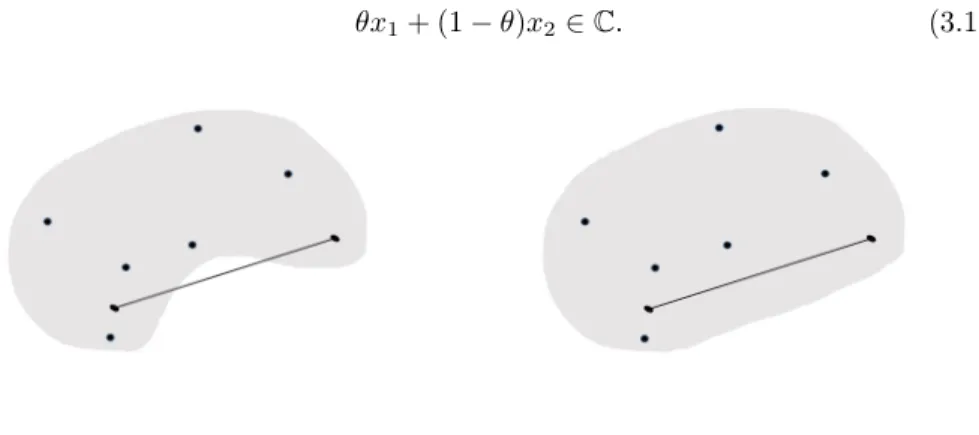
Definition 1. Convex Set

A setCis convex if the line segment between any two points inC lies inC, i.e., if for anyx1, x2∈Cand anyθwith 0≤θ≤1, we have

θx1+ (1−θ)x2∈C. (3.18)

Figure 3.2: Nonconvex Set Figure 3.3: Convex Set

Definition 2. Convex Function

A function f : _Rn _→

R is convex if dom f is a convex set and if for all x, y∈domf, andθ with 0≤θ≤1, we have

f(θx+ (1−θ)y)≤θf(x) + (1−θ)f(y). (3.19) Due to the theory found in the Boyd [3] text, functions defined such as this are found to have unique minimum solutions.

(25)

Figure 3.4: Convex Function f(x) a x _θx_{+ (1}₋_θ₎_y y _b f[θx+ (1−θ)y] θf(x) + (1−θ)f(y) x y

3.5.1 Robust Principal Component Analysis (RPCA)

As discussed in section 3.2, the traditional PCA formulation is known to have the problem of being sensitive to outliers. There has been a significant amount of research over the past decade surrounding Robust Principal Component Anal-ysis(RPCA). [1][2][18] As high dimensional data is now commonplace, it more important than ever to be able to determine the underlying structure hidden in data. At the same time, it is critical to be able to accomplish this despite the presence of sparse gross outliers which do occur in real data for various reasons. While PCA uncovers a low-rank approximation of the original matrix, RPCA differs in that it attempts to separate the original matrix M into an optimal combination of a low-rank matrixL and a sparse matrixS. The sparse matrix that is recovered is not meant to represent small noise, rather it is intended to capture large, sparse outliers. This can be solved as a convex optimization problem. [1]

min||L||∗+λ||S||1s.t.L+S=M (3.20)

In the above optimization problem, the rank constraint is relaxed by utilizing the nuclear norm,||L||∗. As defined in section 3.4.2, minimizing the nuclear norm

will result in a low rank matrix due to sparse singular values. With respect to the matrixS, minimizing the`1 Norm will result in sparse values.

∗ ∗ ∗ ∗ ∗ ∗ ∗ ∗ ∗ ∗ ∗ ∗ ∗ ∗ ∗ ∗ ∗ ∗ ∗ ∗ ∗ ∗ ∗ ∗ ∗ ∗ ∗ ∗ ∗ ∗ ∗ ∗ ∗ ∗ ∗ ∗                   Lis low-rank 0 0 0 0 ∗ 0 0 0 0 0 0 0 0 0 0 0 0 0 0 ∗ 0 0 0 0 0 0 0 0 0 0 0 0 0 ∗ 0 0                   S is sparse (3.21)

(26)

This represents the ideal RPCA and can be achieved by various techniques. Previous research has indicated ideal values forλcan be determined based on the dimensions of the data matrix.[1]

λ= 1/sqrt(max(m, n)) (3.22)

Although the idealλ is useful for optimal recovery ofLandS, that is not the purpose of this research. Inspired by previous work in this area [2], an unsuper-vised approach with the method of varying lambda to adjust the sparsity ofS

will help to find the optimal lambda for the purpose of anomaly detection in DNS data. If a small number of labeled data points are made available, this could become a semi-supervised approach using cross validation techniques to deter-mine optimal threshold values for separating anomalies from normal network data. Success in this area would be noteworthy and could have implications for future solutions to cybersecurity problems.

3.5.2 Sparse PCA

Section 3.5.1 describes a PCA solution that is robust to outliers, however we also seek to address the issue of interpretability. We provide an algorithm for PCA which is robust and improves interpretability. Sparse PCA is formulated as an optimization problem which aims to balance bias and variance by minimizing the loadings on the principal components through the use of a regularization term. It will be shown here that the`1 norm can be used to induce sparsity in

the model while at the same time, the `2,1 norm will provide sparsity in the

features. Previous work in this area can be traced back to a maximum variance approach of Jolliffe et al. called Simplified Component Technique-LASSO (SCoTLASS) [20] as well as an approach which minimizes error by Zou et al. [19] The maximum variance approach is as follows.

maxvT(XTX)v, subject to

p X j=1

|vj| ≤t, vTv= 1 (3.23)

The minimize error approach is shown here.

minθ,v N X i=1 kxi−θvTxik22+λkvk 2 2+λ1kvk1 subject tokθk2= 1 (3.24)

Further details of the above research can be found in [15][20]. Inspired by the previous methods, we present the following Sparse PCA formulation which combines both the`2,1norm and the`1norm and is expressed as the following

optimization problem. min

A,S||X−AX−S|| 2

(27)

This formulation is similar to RPCA in that it uncovers a low-rank matrix and a sparse matrix. However, the key differentiator in this model is that the low-rank matrix is comprised of a structurally sparse representation of the original matrix. What this means is that it is sparse in the columns and therefore more interpretable because it translates into sparse features.

0 0 0 0 0 0 0 0 0 0 0 0                   · · · col1col2 colm

Ahas some columns = 0

0 0 0 0 ∗ 0 0 0 0 0 0 0 0 0 0 0 0 0 0 ∗ 0 0 0 0 0 0 0 0 0 0 0 0 0 ∗ 0 0                  

SparseS contains outliers

(3.26)

As discussed in 3.4, the regularization parameters must be tuned to balance the bias and variance in the model. This is a difficult aspect of any optimization problem and must be carefully analyzed. The methods used for tuningλandφ

in our Sparse PCA formulation will be discussed in Chapter 5.

3.6 Non-Linear Approaches

3.6.1 The Kernel Trick

It is often the case that data cannot be separated into classes with a linear boundary. One method for dealing with non-linearity is to transform the data into a new (often higher dimensional) space such that the classes are linearly separable in the new space. A key solution in the machine learning world is called theKernel Trick, and is based on Mercer’s Theorem. Explicitly defining Mercer’s Theorem here would take us too far astray, however details can be found in many sources such as the data mining textbook cited here. [5] In basic terms, following closely from the Wikipedia description [22], given a non-linear mapping function ϕ, data can be transformed into a new space in which a linear boundary exists. For allx andx0 in the input spaceX, some functions

k(x, x0) can be written as aninner product in another space V. The kernel is written as a feature mapϕ:X → V where

k(x, x0) =hϕ(x), ϕ(x0)iv.

In order to be valid, h., .iv must be a proper inner product. If a kernel is established to be valid, then one can conclude that the feature space of data in that kernel exists even if we do not know exactly what that space is. This is

(28)

very powerful because it allows us to find a feature space in which our data is linearly separable.

3.6.2 Kernel Principal Components Analysis (KPCA)

Kernel PCA allows for non-linear separation of data through the use of a kernel trick. As described in the previous section 3.6.1, data can be mapped to a new feature space using a kernel function. Linear PCA is then performed in that higher dimensional space. Because the feature space may be very high dimension (in fact, it could be infinite dimensional), the kernel trick is used and KPCA is computed on the kernel matrix. [14] Although we will not cover Kernel functions extensively in this document, it should be noted that the cosine function satisfies the conditions of Mercer’s Theorem and can therefore be used to perform Kernel PCA. The cosine function is discussed further in section 3.6.3

3.6.3 Cosine Function Background

The cosine function has properties which turn out to be useful for machine learning and the use of the kernel trick. Specifically, having a similarity function depending on the angle rather than the length of two vectors allows for a different way to discover non-linear structure. Cosine similarity is a measurement of the angle between two vectors. If the angle between x and y is zero degrees then the cosine similarity is equal to one. It does not matter if the magnitude (lengths) of x and y are different. [5] The cosine function is defined as follows

cos(x, y) = x·y

||x|| ||y|| (3.27)

(29)

Chapter 4 RPCA Experiments and

Results

4.1 Data Description

For the purpose of this research, a large set of anonymized computer network data was made available through collaboration with The MITRE Corporation in Bedford, Massachusetts. Previous work done at MITRE involved a similar study of sizeable network data containing a small number of data points labeled as anomalies. [2] New research efforts will build upon previous work and move forward in new directions with the goal of discovering novel methods for anomaly detection in DNS data. The original dataset consists of 118 DNS splunk logfiles in .csv file format. Each file spans about 30 seconds in time. In total, the entire data set represents millions of rows of data captured over the course of one hour which were then parsed and saved as client vs query matrices as described below. In order to avoid data snooping, 18 of the original files were chosen at random and set aside as holdout data. This left a remainder of 100 files to analyze. These were split at random into a set of 20 test files and 80 training files. In order to avoid overfitting, 40 of the training files were altered slightly by removing 20% of rows at random.

Due to the complex nature of the data, and to avoid the Curse of Dimension-ality, initial data analysis was performed utilizing just two features of primary interest. These two features were the client IP address and the domain name which was attempted to be resolved. Matrices were assembled indicating clients vs queries and the counts of occurrences of each.

A critical step in the process of building the client vs query matrices was the identification of specific blacklisted queries which were used for label-ing some of the data as anomalous. This detection of blacklisted queries was a key discovery which enabled some form of semi-supervised learning to be done.

(30)

4.2 Data Challenges

There are two obvious challenges with this data.

• Very few labeled anomalies (Imbalanced classes)

• Sparsity of original matrix

These limitations mean that traditional approaches to RPCA may not be ad-equate. Furthermore, it may be determined that methods other than RPCA may be more suitable for data with such properties. It is clear that the opti-mization of lambda alone is not going to be adequate for the accurate detection of anomalies in this data. Some of the limitations with the data will require the creation of a set of decision rules to determine a threshold parameter which will further define the feature vectors in the matrices. These features can then be passed to traditional classification algorithms (such as a Random Forest) and cross validation can be used to determine the best lambda and threshold values. The issues of class imbalance and data sparsity are described in further detail below. These make for a very difficult problem to solve, however if accurate techniques are discovered this would be considered groundbreaking work in the field.

4.2.1 Imbalanced Data

As a binary classification problem, each query can be labeled as blacklisted = TRUE or blacklisted = FALSE. A data set is said to be imbalanced when the class distribution has an excessive amount of data labeled as one class compared to another. [5] As an exmple, consider a dataset of 1 Million DNS queries where 99.5% (or 995,000) are labeled FALSE and just 0.5% (5,000) are labeled TRUE anomalies. This is the level of imbalance seen in our data and is not uncommon for many real world data sets involving network logs analyzed for cybersecurity. Class imbalance problems are often likened to ”finding a needle in a haystack”. Fortunately, there are some techniques for artificially balancing the data in order to ease the analysis. It will be important to explore various sampling based approaches to artificially balance the data. Details regarding balancing the data will be described in sections below.

4.2.2 Sparse Data

Attempted classification on sparse data presents many challenges. This type of problem is not unique to computer network data. Real world problems involving classification of text documents is a frequently cited example. The sparsity of the original matrix for the purpose of utilizing RPCA will be one of the challenges this research will need to address.

(31)

4.2.3 Accuracy Measures and Sampling

When dealing with imbalanced data, the traditional performance measure of accuracy may be an inadequate measure of performance. Binary classification problems often use the metrics of a confusion matrix to measure prediction performance. However, due to the imbalanced nature of the data, the pre-ferred method for measuring accuracy takes into consideration the measures of precision and recall. The Receiver Operating Characteristic (ROC) Curve is a common visual technique often used for graphical analysis detecting rare classes. [5]

4.3 RPCA on Original Data

Shown here, is a graphical representation of the original matrixX where the x axis represents queries that were attempted and the y axis represents individual clients making those queries.

Initial attempts were made as described previously with respect to fine tuning

Figure 4.1: Client VS Query Matrix

the lambda parameter in the optimization problem. A range of lambda values in the RPCA calculation resulted in

• a very small lambda which put most of the data into the sparse matrix S

• a very large lambda which essentially put all of the data into the low rank matrix L, but nothing ended up in the sparse matrix S.

(32)

Resulting low-rank matrix L and sparse matrix S for a smalllambda:

(33)

4.4 PCA on Original Data

The following plots serve as a visual baseline to demonstrate the value of preprocessing. As a first step, PCA was performed on one of the original matrices (before normalization).

4.5 PCA on Data Normalized with

Standard-Scaler

Preprocessing data by normalization is a critical step before applying most machine learning algorithms. The python package, scikit-learn, provides a StandardScaler method which is a standard z score normalization.

(34)

4.6 PCA

on

Data

Normalized

with

Ro-bustScaler

Oftentimes, when many outliers are present, scaling using the mean and variance of the data is found to be inadequate. The python scikit-learn package offers a solution for this with its RobustScaler which uses robust estimates for data center and range instead. The following plots demonstrate PCA on data scaled with the RobustScaler method.

(35)

4.7 PCA on Balanced Data

Data analysis is also complicated by the fact that the data is very imbalanced. Only approximately 80 of the 60,000 queries in each matrix (0.1%) is labeled as anomalous (denied due to blacklist status). This was observed to be consistent across the 100 matrices. Therefore, analysis of a single matrix was deemed to be appropriate for initial experiments. The following plots demonstrate PCA results after various levels of stratification. As can be seen by the ROC Curve, balancing the data provides significant improvement.

(36)

4.8 RPCA on Balanced Data

After realizing the positive effects of balancing the data, RPCA was attempted on a balanced data set. Surprisingly, this revealed anomalies in the low-rank matrix and normal DNS data in the sparse matrix. Previous work that was done in this area presumed the opposite, and experiments had poor results. Further analysis on this remains to be done to confirm this and to perform better fine-tuning of the RPCA lambda parameter.

(37)

In the plots provided here, the lower half of the matrices contain the rows where the anomalous queries exist. Very small values of lambda pushed all of the data into the sparse matrix S. Very large values of lambda pushed everything into the low-rank matrix L. For a lambda somewhere in the middle, blacklisted queries appear to reside in L and normal queries in S.

(38)

4.9 Kernel PCA with Cosine Results

Kernel PCA utilizing the cosine function demonstrates remarkable results. These plots of principal components reveal distinct separation of data that was once so intermixed that points were not able to be classified. Stratification was initially one-to-one, but upon inspection of up to 200-to-1 balancing, the results remain the same. The Cosine KPCA appears to separate the classes. The dark points are training and the light points are test data. (Dark Blue = Normal Train, Light Blue = Normal Test, Dark Red = Anomaly Train, Light Red = Anomaly Test)

(39)

Chapter 5 Sparse PCA Experiments

and Results

5.1 Data

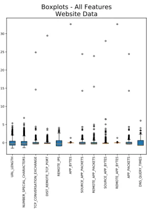
For the purpose of demonstrating the Sparse PCA technique described in section 3.5.2, we make use of a dataset consisting of approximately 1500 websites each characterized by the following twelve features

Furthermore, each sample is labeled True or False indicating whether or not the website is malicious. The data set can be found on the Kaggle platform along with a paper describing previous research. [21]. A boxplot of normalized features, seen in Figure 5.1, provides a first glance at the data.

(40)

URL_LENGTH

NUMBER_SPECIAL_CHARACTERS TCP_CONVERSATION_EXCHANGE

DIST_REMOTE_TCP_PORT

REMOTE_IPS APP_BYTES

SOURCE_APP_PACKETS REMOTE_APP_PACKETS SOURCE_APP_BYTES REMOTE_APP_BYTES

APP_PACKETS DNS_QUERY_TIMES 0 5 10 15 20 25 30

Boxplots - All Features

Website Data

Figure 5.1: Boxplots - All Features

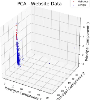
An initial exploratory anlaysis utilizing PCA on normalized data z-scored by features (see Figure 5.2), reveals there will be some difficulty classifying these sites utilizing traditional techniques. The red dots in the plot indicate malicious sites. They are so intermixed with the benign sites that they are difficult to see in the plot.

(41)

Principal Component 1

0 10 20 30 40 50 20

_{Principal Component 2}

100 1020 30

Principal Component 3

2 0 2 4 6

PCA - Website Data

Malicious Benign

Figure 5.2: PCA - Website Data

A plot of explained variance (Figure 5.3), however, gives us some hope that the data has a low rank as most of its variance can be explained with just a few principal components.

(42)

0 2 4 6 8 10 Principal Components 0.5 0.6 0.7 0.8 0.9 1.0

Percent of Explained Variance

PCA Cumulative Explained Variance Website Data, All Features

Figure 5.3: Cumulative Explained Variance - All Features

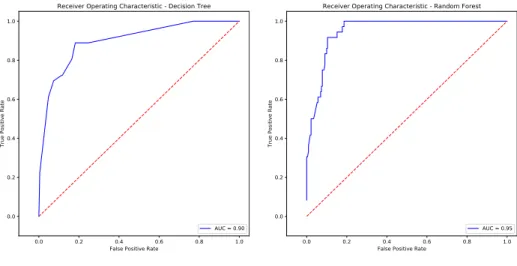
We provide here, some results of traditional machine learning classifiers fit on the dataset so that we might compare results to our proposed Sparse PCA model.

URL_LENGTH

APP_PACKETS DNS_QUERY_TIMES 0.00 0.05 0.10 0.15 0.20

Feature ranking - Random Forest

Figure 5.4: Random Forest

URL_LENGTH

APP_PACKETS DNS_QUERY_TIMES 0.00 0.05 0.10 0.15 0.20

Feature ranking - Decision Tree

(43)

0.0 0.2 0.4 0.6 0.8 1.0 False Positive Rate

0.0 0.2 0.4 0.6 0.8 1.0

True Positive Rate

Receiver Operating Characteristic - Decision Tree

AUC = 0.90

Figure 5.6: Decision Tree ROC

0.0 0.2 0.4 0.6 0.8 1.0

False Positive Rate 0.0 0.2 0.4 0.6 0.8 1.0

True Positive Rate

Receiver Operating Characteristic - Random Forest

AUC = 0.95

Figure 5.7: Random Forest ROC

5.2 Methods

Recall the Sparse PCA formulation (3.25).

minimizeA,S||X−AX−S||2F+λ||A||2,1+φ||S||1

We will show how this technique enables us to reduce dimensionality by elim-inating some features while at the same time, separating outliers. Before we proceed to explain how we go about tuning our model parameters, it is worth noting there are two easy solutions to the model.

1. A=I andS= 0 2. A= 0 and S=X

We are not interested in the simple solutions enumerated above as we seek to find a balance of an interpretable low-rankA and a sparse matrix of outliers,

S. In order to accomplish this we will tuneλandφ.

Tuning model parameters can be a tedious process. If we focus solely on the dimensionality reduction (i.e. set the regularization parameter φ = 0 in equation (3.25)) we find that as λ increases, the mean squared error of our objective function increases as shown in Figure 5.2.

(44)

0 1000 2000 3000 4000 5000 Lambda 0.0 0.2 0.4 0.6 0.8 1.0

Mean Squared Error of (X-AX)

Effect of lambda on Error when phi = 0

Figure 5.8: Effect of lambda on MSE

Based on Figure 5.2 we might select an initial lambda value to be 500 and then holding that value stable we see how changing phi impacts the error in the model. 3.00 3.25 3.50 3.75 4.00 4.25 4.50 4.75 Phi 21.8 21.9 22.0 22.1 22.2 22.3 22.4 22.5

Mean Square Error of (X - AX - S)

Effect of phi on Error when lambda=500

Figure 5.9: Effect of phi on MSE when lambda=500

However, if we simply set λ = 0 and φ = 0 we obtain the solution for minimizing our mean squared error term, kX −AXk2

F to be that A is the

identity matrix,A=I. We must make use of the regularization termλkAk2,1

in order to eliminate some features by producing sparsity in the columns. Another set of plots are shown in Figure 5.2 which could be useful for tuning the

(45)

model involve plotting various outcomes with respect toλandφ. For example, it is helpful to see how many columns in our model matrixA become zeroed out, or how many data points end up in the matrixS.

150 152 154 156 158 Lambda 0.0 0.2 0.4 0.6 0.8 1.0 Phi 0 0 2 4 4 4 7 7 7 9 9 7 8 8 8 8 8 8 8 8 0 0 2 4 4 4 7 7 7 8 9 7 8 8 8 8 8 8 8 8 0 0 2 4 4 4 7 7 7 8 9 7 8 8 8 8 8 8 8 8 0 0 2 4 4 4 6 7 7 8 9 9 8 8 8 8 8 8 8 8 0 0 2 4 4 4 6 7 7 8 9 9 8 8 8 8 8 8 8 8 0 0 2 4 4 4 6 7 7 8 9 9 8 8 8 8 8 8 8 8 0 0 2 4 4 4 6 7 7 8 9 9 7 8 8 8 8 8 8 8 0 0 2 4 4 4 6 7 7 8 9 9 7 8 8 8 8 8 8 8 0 0 2 3 4 4 6 7 7 8 9 9 7 8 8 8 8 8 8 8 0 0 2 3 4 4 6 7 7 8 9 9 7 8 8 8 8 8 8 8

Effect of lambda and phi on Number of nonzero columns of A

(features selected)

Figure 5.10: Columns Remaining in A

150 152 154 156 158 Lambda 0.0 0.2 0.4 0.6 0.8 1.0 Phi 3617 3361 2773 2143 1729 1391 1104 854 648 474 370 282 228 190 149 133 115 105 97 87 3617 3362 2788 2170 1734 1396 1116 864 650 488 376 286 233 194 155 133 116 105 97 87 3617 3362 2793 2177 1733 1399 1126 875 660 494 381 286 235 194 157 133 117 106 98 88 3617 3362 2806 2178 1735 1403 1133 887 667 498 383 289 237 194 160 138 119 108 99 88 3617 3361 2832 2191 1762 1411 1139 895 672 502 394 292 240 197 161 138 119 111 100 91 3617 3362 2841 2198 1764 1414 1146 901 681 515 397 300 247 200 166 139 119 112 100 92 3617 3362 2856 2217 1765 1424 1154 904 688 522 401 304 248 202 168 140 121 112 100 93 3617 3362 2830 2225 1774 1432 1159 912 702 525 405 306 255 202 171 140 123 112 101 95 3617 3362 2886 2223 1786 1435 1167 925 706 531 410 317 256 208 172 140 124 112 102 95 3617 3361 2891 2234 1828 1438 1171 931 711 544 418 320 257 211 174 141 125 112 104 97

Effect of lambda and phi on data points in S (outliers detected)

Figure 5.11: Data Points In S While all of the above plots were are helpful in tuning the regularization parameters, it is still a tedious process that requires more intuition. Data visu-alization of the process is a critical component. Specifically, three-dimensional plots are most beneficial in combination with a novel scoring method described here. The ’perfect’ solution to a regularized optimization problem depends com-pletely on the desired degree of bias and variance for the particular problem at hand. Furthermore, a model may require parameters to be tuned on a case by case basis. Consider the data set at hand. We wish to reduce dimensionality in a structured manner while separating some degree of outliers. A scoring method is presented here which allows λto be tuned based on how many features we would like to retain. At the same time, phi can be tuned based on level of sparsity desired in outliers removed. The scoring method in combination with the three dimensional plots allow for this visual inspection of the bias variance tradeoff for our specific data set. The scoring method corresponds directly to the model formulation (3.25) and is as follows.

ModelScore = Least Squares Term + Column Term + Outlier Term Where

1. Least Squares Term =kX−AX−Sk

2. Column Term =|Columns in A - Desired Number of Columns in A|

(46)

Figure 5.12: Least Squares component of Model Score. The least squared error term rises quickly asλincreases.

(47)

Figure 5.13: Number of Features component of Model Score. The number of columns not zeroed out by the`2,1norm in the formulation. Although this plot

doesn’t cover the full range ofλandφrequired to view all combinations, it can be seen that there are more possibilities for some combinations than others.

(48)

Figure 5.14: Outlier component of Model Score. The norm of S is seen to be quite large whenφis small. As soon as φis big enough, the penalty for items in S is sufficient to keep the matrix (and therefore, its norm) small.

Finally, a plot comprised of the three components of the score can be utilized. 5.2

(49)

Figure 5.15: Total Model Score. This plot demonstrates what happens to the total score asλandφchange. The total score is the sum of the three components seen in 5.2, 5.2 and 5.2.

5.3 Interpreting Results

One main result of the Sparse PCA method is the ability to separate data into interpretable and structured low rank form with outliers removed. Even with a small dataset as demonstrated here, it quickly becomes cumbersome to experiment. For example, given nfeatures and k desired features to measure, there are n_k

combinations.

To demonstrate measurable results of the Sparse PCA model, we provide examples of dimensionality reduction on the website dataset. Recall that the original dataset has 12 features for each website sample. Here are the results demonstrating robust sparse solutions for various reduced sets of features. We then compare these results to Receiver Operating Characteristic Plots where the same features were manually eliminated and then analyzed with the same machine learning algorithms. We discover comparable results, indicating that

(50)

our Robust Sparse PCA solution may be able to replace a brute force and often computationally expensive approach.

URL_LENGTH

REMOTE_IPS

REMOTE_APP_PACKETS SOURCE_APP_BYTES DNS_QUERY_TIMES 0 5 10 15 20 25 Boxplots - 7 Features Website Data

Figure 5.16: Boxplot, 7 Features

0.0 0.2 0.4 0.6 0.8 1.0

True Positive Rate

AUC = 0.85

(51)

0.0 0.2 0.4 0.6 0.8 1.0

True Positive Rate

AUC = 0.92

Figure 5.18: ROC, RSPCA 7 Features RF

0.0 0.2 0.4 0.6 0.8 1.0

True Positive Rate

Receiver Operating Characteristic - RBF SVM

AUC = 0.86

(52)

0.0 0.2 0.4 0.6 0.8 1.0

True Positive Rate

AUC = 0.84

Figure 5.20: ROC, 7 Manually Selected Features DT

0.0 0.2 0.4 0.6 0.8 1.0

True Positive Rate

AUC = 0.94

(53)

0.0 0.2 0.4 0.6 0.8 1.0

True Positive Rate

AUC = 0.86

Figure 5.22: ROC, RSPCA 7 Manually Selected Features SVM

URL_LENGTH NUMBER_SPECIAL_CHARACTERS TCP_CONVERSATION_EXCHANGE DIST_REMOTE_TCP_PORT REMOTE_IPS REMOTE_APP_PACKETS SOURCE_APP_BYTES DNS_QUERY_TIMES 0 5 10 15 20 25 30 Boxplots - 8 Features Website Data

(54)

0.0 0.2 0.4 0.6 0.8 1.0

True Positive Rate

AUC = 0.89

Figure 5.24: ROC, RSPCA 8 Features DT

0.0 0.2 0.4 0.6 0.8 1.0

True Positive Rate

AUC = 0.96

(55)

0.0 0.2 0.4 0.6 0.8 1.0

True Positive Rate

AUC = 0.86

Figure 5.26: ROC, RSPCA 8 Features SVM

0.0 0.2 0.4 0.6 0.8 1.0

True Positive Rate

AUC = 0.90

(56)

0.0 0.2 0.4 0.6 0.8 1.0

True Positive Rate

AUC = 0.97

Figure 5.28: ROC, 8 Manually Selected Features RF

0.0 0.2 0.4 0.6 0.8 1.0

True Positive Rate

AUC = 0.86

(57)

Chapter 6 Conclusions

6.1 Contributions

In this work we have examined methods for dimensionality reduction resulting in arbitrary low-rank solutions capturing maximum data structure as well as alternative methods resulting in structured low-rank solutions which are highly interpretable with respect to data features. Both approaches are improved by the addition of the Least Absolute Shrinkage and Selection Operator Norm for the purpose of increasing robustness of the models. Methodologies for regular-ization parameter tuning were presented as well. These novel methods are both scalable with respect to data and extensible in a variety of domain applications.

6.2 FutureWork

This work can be applied to many domains. Future work could focus on a number of different areas including examining how the methods scale, pushing the boundaries of work done here to include non-linear interpretations, as well advancements in the data visualization component of tuning the optimization problem.

1. Big Data - Experiment on really high dimensional data

2. Deep Learning - Define in non-linear methods for use with neural networks 3. Data Visualization - Use advanced data visualization for model tuning

(58)

Bibliography

[1] Cands, Emmanuel J. et al. Robust principal component analysis? J. ACM 58 (2011): 11:1-11:37.

[2] Paffenroth, Randy et al. Robust PCA for Anomaly Detection in Cyber Networks. CoRR abs/1801.01571 (2018): n. pag.

[3] Boyd, S., Vandenberghe, L. (2004). Convex Optimization. Cambridge University Press. ISBN: 0521833787

[4] Reducing the Dimensionality of Data with Neural Networks, G.E. Hinton and R.R. Salakhutdinov, Science 313, 504 (2006)

[5] Tan, P.-N., Steinbach, M.,, Kumar, V. (2006). Introduction to Data Mining. Addison Wesley.

[6] Whitehouse,

https://www.whitehouse.gov/wp-content/uploads/2018/02/ap 21 cyber security-fy2019.pdf

[7] Threat Intelligence and Analytics 2010-2017 ICT Market Review and Forecast, available at : http://test.tiaonline.org/resources/market-forecast

[8] International Data Corporation, Worldwide

Semian-nual Security Spending Guide, October 12, 2016, at

www.idc.com/getdoc.jsp?containerId=prUS41851116.

[9] Two Shady Men Walk Into a Bar, Detecting Suspected Malicious In-frastructure Using Hidden Link Analysis, RecordedFuture available at : http://go.recordedfuture.com/hubfs/reports/two-shady-men.pdf

(59)

[10] Sucuri’s Hacked Website Report at https://sucuri.net/reports/2016-q2-hacked-website-report

[11] Eckart, C. and Young, G. Psychometrika (1936) 1: 211. https://doi.org/10.1007/BF02288367

[12] Stewart, G. W. (1993). ”On the Early History of the Singular Value Decomposition”. SIAM Review. 35 (4): 551566. doi:10.1137/1035134. JSTOR 2132388.

[13] Petruccelli, J., Nandram, B., Chen, M., (1999). Applied Statistics for Engineers and Scientists, Pearson p. 157

[14] Gareth James, Daniela Witten, Trevor Hastie, Robert Tibshirani. (2013). An Introduction to Statistical Learning : With Applications in R. New York :Springer

[15] Hastie, T., Tibshirani, R.,, Friedman, J. (2001). The Elements of Statistical Learning. New York, NY, USA: Springer New York Inc..

[16] W.B. Johnson and J. Lindenstrauss, Extensions of Lipschitz mappings into a Hilbert space, Contemporary Mathematics, 26, (1984)

[17] Sanjoy Dasgupta and Anupam Gupta, An Elementary Proof of a Theorem of Johnson and Lindenstrauss, 2003, Wiley Periodicals Inc., Random Struct. Alg. 22: 60-65, 2002

[18] Wright, John et al. Robust Principal Component Analysis: Exact Recovery of Corrupted Low-Rank Matrices via Convex Optimization. NIPS (2009).

[19] Zou H, Hastie T, Tibshirani R. 2006 Sparse principal components J. Comput. Graph. Stat. 15, 262-264 (doi:10.1198/jcgs.2006.s)

[20] Ian Jolliffe, Nickolay Trendafilov, Mudassir Uddin, ”A Modified Principal Component Technique Based on the LASSO”, 2003 American Statistical Association, Institute of Mathematical Statistics, and Interface Foundation of North America. Journal of Computational and Graphical Statistics, Volumne 12, Number 3, Pages 531-547 DOI: 10.1198/1061860032148

(60)

[21] Urcuqui, C., Navarro, A., Osorio, J., Garca, M. (2017). Machine Learning Classifiers to Detect Malicious Websites. CEUR Workshop Proceedings. Vol 1950, 14-17.

[22] Wikipedia online mathematical definition of Kernel Method found at : https://en.wikipeda.org/wiki/Kernel method

Dimension Reduction and LASSO using Pointwise and Group Norms

Worcester Polytechnic Institute

Digital WPI

Masters Theses (All Theses, All Years)

Electronic Theses and Dissertations

2018-12-11

Dimension Reduction and LASSO using

Pointwise and Group Norms

Melanie A. Jutras

Follow this and additional works at:

https://digitalcommons.wpi.edu/etd-theses

Repository Citation

WORCESTER POLYTECHNIC INSTITUTE

Dimension Reduction and LASSO

using

Pointwise and Group Norms

December 2018

Contents

Abstract

Executive Summary

Acknowledgments

Chapter 1

Introduction

1.1

Previous Work

1.2

Novel Contributions

1.3

Organization

Chapter 2

Motivation

2.1

Broad Applicability to Many Domains

2.2

Application to Cybersecurity Domain

2.2.1

Security is Expensive

2.2.2

Security is Hard

2.2.3

DNS Data Background

Chapter 3

Methodology

3.1

Dimensionality Reduction

3.2

Principal Components Analysis (PCA)

3.2.1

PCA as an Eigendecomposition

3.2.2

Singular Value Decomposition

3.2.3

Eckart-Young

3.3

Standardization

3.4

Regularization

3.4.1

Unregularized Least Squares

3.4.2

Norms

3.4.3

Ridge Regression

3.4.4

LASSO

3.5

Convex Optimization Problems

3.5.1

Robust Principal Component Analysis (RPCA)

3.5.2

Sparse PCA

3.6

Non-Linear Approaches

3.6.1

The Kernel Trick

3.6.2

Kernel Principal Components Analysis (KPCA)

3.6.3

Cosine Function Background

Chapter 4

_{Principal Component 2}