Federal Reserve Bank of Minneapolis Research Department StaffReport 432 Revised February 2012
Consumption and Labor Supply with Partial Insurance:
An Analytical Framework
∗Jonathan Heathcote
Federal Reserve Bank of Minneapolis and CEPR
Kjetil Storesletten
Federal Reserve Bank of Minneapolis, University of Oslo,
and CEPR
Giovanni L. Violante New York University, CEPR,
and NBER [email protected]
ABSTRACT
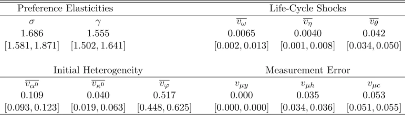
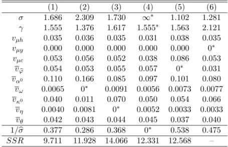
This paper develops a model with partial insurance against idiosyncratic wage shocks to quantify risk sharing, and to decompose inequality into life-cycle shocks versus initial heterogeneity in preferences and productivity. Closed-form solutions are obtained for equilibrium allocations and for moments of the joint distribution of consumption, hours, and wages. We prove identification and estimate the model with data from the CEX and the PSID over the period 1967—2006. We find that (i) 40% of permanent wage shocks pass through to consumption; (ii) the share of wage risk insured privately increased until the early 1980s and remained stable thereafter; (iii) life-cycle productivity shocks account for half of the cross-sectional variance of wages and earnings, but for much less of dispersion in consumption or hours worked.
∗Heathcote and Violante’s research is supported by a grant from the National Science Foundation (SES 0418029). Storesletten thanks the Research Council of Norway and the Centre of Equality, Social Orga-nization, and Performance. The views expressed herein are those of the authors and not necessarily those of the Federal Reserve Bank of Minneapolis or the Federal Reserve System.
1
Introduction
How effectively can households smooth idiosyncratic wage fluctuations via private insurance arrangements and labor supply adjustments? To what degree has the four-decade-long rise in US wage dispersion passed through to inequality in consumption and hours worked? More broadly, what is the role of uninsurable life-cycle shocks to wages relative to initial heterogeneity in skills and preferences in accounting for observed inequality? The purpose of this paper is to measure the degree of risk sharing achieved by US households, and to examine how it has changed over the past forty years. Quantifying the extent of private risk sharing is important in determining the appropriate role for redistributive taxation and public insurance programs.
The measurement of risk sharing has been approached in two ways in the existing lit-erature. The first approach is to build a structural equilibrium model, and to use it as an artificial laboratory to study the response of consumption to individual income fluctua-tions. One prominent example is the standard incomplete-markets model, where households self-insure against income fluctuations by borrowing and lending via a risk-free bond (see Heathcote, Storesletten, and Violante (2009) for a survey). The key limitation of the struc-tural approach is that the amount of risk sharing in the model is always sensitive to the model assumptions regarding the asset market structure and the insurance channels available to agents.
The alternative approach in the literature is to quantify the overall degree of insurability of income innovations, while remaining somewhat agnostic about the specific sources of risk sharing. Deaton (1997) pioneered this methodology.1 An important recent example of this less structural approach to measuring insurance is Blundell, Pistaferri, and Preston (2008), who use longitudinal data on income and consumption (constructed through an imputation procedure) to estimate the degree to which permanent changes in earnings pass through to household consumption. This methodology requires a long panel of high-quality income
1Deaton (1997, pp. 372-374) writes: “Saving is only one of the ways people can protect their consumption
against fluctuations in their income. An alternative is to rely on other people, to share risk with friends and kin, with neighbors, or with other anonymous participants through private or government insurance schemes, or through participation in financial markets ... [T]he very multiplicity of existing mechanisms makes it likely that there is at least partial insurance through financial or social institutions, and that such risk sharing adds to the possibilities for autarkic consumption smoothing through intertemporal transfers of money or goods ... Although it is possible to examine the mechanisms, the insurance contracts, tithes and transfers, their multiplicity makes it attractive to look directly at the magnitude that is supposed to be smoothed, namely consumption.”
and consumption data. Moreover, the estimation procedure embeds assumptions on the equilibrium process for consumption, and pass-through coefficients will be biased if these assumptions are not satisfied (see Kaplan and Violante (2010) for a discussion).
This paper pursues a new approach to measuring risk sharing that combines elements from both these traditions. We estimate the overall amount of private consumption insurance in the context of a structural equilibrium model that allows for a flexible financial market structure – and thus does not “hardwire” agents’ access to insurance. Our framework is an augmented version of the standard incomplete-markets model with idiosyncratic wage risk. We assume isoelastic preferences over consumption and hours worked, and allow for heterogeneity in the taste for work. Wages have two orthogonal stochastic components, which we label (privately) “insurable” and “uninsurable,” respectively. Agents can perfectly smooth the “insurable” component. The “uninsurable” component can only be smoothed via adjustments to own hours worked, via government redistribution, or through borrowing and lending in a riskless bond.
The equilibrium allocations of consumption and hours emerging from our framework can be expressed in closed form, as log-linear functions of the idiosyncratic distaste for work and of the two wage components. An important step toward characterizing allocations is to show that in equilibrium the bond is not used to smooth “uninsurable” shocks – a result that extends the logic in Constantinides and Duffie (1996) to a much richer environment. The analytical derivation of allocations is the first theoretical contribution of the paper.
These closed-form log-linear allocations make it possible to compute and interpret cross-sectional variances and covariances of the joint equilibrium distribution of wages, hours, and consumption. We use information contained in both the “macro facts” on the distributions of these variables in levels that have motivated recent macroeconomic investigations (e.g., Attanasio and Davis, 1996; Krueger and Perri, 2006; Heathcote, Storesletten, and Violante 2010b), and the “micro facts” on the distributions ingrowth rates that have been the primary focus of labor economists (e.g., Abowd and Card, 1989; Blundell, Pistaferri, and Preston, 2008). The analytical expressions for these cross-sectional moments allow us to formally prove identification of all the model’s parameters given standard micro data sets – something that is usually impossible in large scale structural models. Proof of identification is our second theoretical contribution.
Most of the literature on risk sharing focuses on how labor market shocks transmit to consumption (see Jappelli and Pistaferri (2010) for a recent survey). We argue that data on
labor supply are also informative about the degree of insurance, because theory predicts that households should adjust hours more strongly in response to insurable versus uninsurable wage increases, reflecting the absence of offsetting wealth effects in the former case. We prove that the model is in fact fully identified given only panel data on wages and hours worked, i.e., without any consumption data. Given uncertainty about the quality of self-reported consumption expenditures (e.g., Attanasio, Battistin, and Ichimura, 2007; Aguiar and Bils, 2011), it is useful to be able to estimate insurance without using consumption data, and to assess whether estimates of insurance derived from wage and hours data alone are consistent with those that use consumption moments. Exploiting moments involving hours worked to quantify risk sharing is our third contribution.
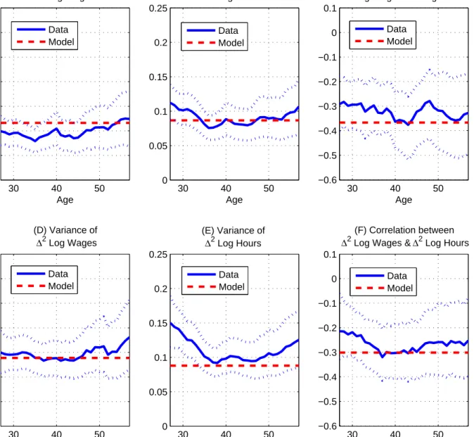
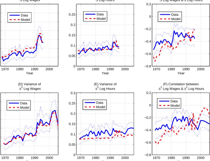
We estimate the model using data on wages and hours from the Panel Study of Income Dynamics (PSID) over the period 1967-2006, and consumption data from the Consumer Expenditure Survey (CEX) over the period 1980-2006. The estimated model replicates well the evolution of the empirical cross-sectional distribution over wages, hours worked and consumption, both over time and over the life cycle. The estimated value for the intertemporal elasticity of substitution for consumption is 1/1.56,while the Frisch elasticity of labor supply with respect to pre-tax wages is 0.38. We estimate significant heterogeneity in the distaste for work, which is needed to account for the observed joint distribution over consumption and hours worked. The estimation also recovers time series for the insurable and uninsurable fractions of wage dispersion, which allow us to address the three questions that motivate our investigation.
First, we ask how much individual wage risk can be smoothed, and what are the relative contributions to smoothing of private risk sharing, government-provided insurance, and la-bor supply adjustments. Blundell, Pistaferri, and Preston (2008) argue that a natural way to measure consumption insurance is to quantify how much of a typical permanent shock to wages passes through to consumption. Our model suggests that this pass-through coeffi-cient is around 40%, or equivalently that 60% of permanent wage fluctuations are effectively smoothed. Where does this insurance come from? Half reflects private risk sharing, one-third reflects progressive taxation, and the rest reflects adjustments to labor supply. A caveat is in order. A common alternative metric for consumption smoothing in the literature is the ratio of the within-cohort change in the variance of log consumption to the corresponding change in the variance of log income (e.g., Blundell and Preston, 1998; Storesletten, Telmer, and Yaron, 2004a). In our framework the two measures of insurance coincide only when
pro-gressive taxation and labor supply are absent as insurance channels. Our baseline parameter estimates indicate a significantly smaller value for the ratio-of-variances statistic than for the pass-through coefficient.
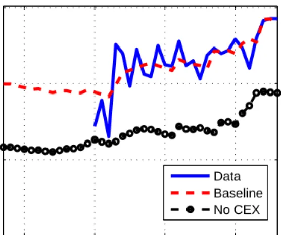
Second, we ask how risk sharing has changed over time. We find that US households were effectively able to insure two-thirds of the sharp increase in wage inequality over the past 40 years. Private risk sharing increased during the 1970s: in 1967 the insurable component of wages accounted for around 25% of the cross-sectional variance of log wages, while by the early 1980s this fraction was around 45%. Since then, the variances of the insurable and uninsurable components of wages have risen at a similar rate, leaving the fraction of wage fluctuations insured relatively stable. Data on hours worked are an essential input for these estimates, since no consumption data in available prior to 1980, and it is the observed increase in the covariance between wages and hours that indicates an increase in the degree of risk sharing. Reassuringly, after 1980, data on hours worked and data on consumption deliver consistent estimates for the relative importance of insurable and uninsurable shocks. Third, we use the estimated model to decompose inequality in the cross section into com-ponents reflecting life-cycle shocks versus initial heterogeneity in productivity and the disu-tility of work effort. This decomposition is unique and additive in our framework. Roughly half of the total cross-sectional variance in wages and earnings reflects life-cycle shocks to wages. In contrast, these shocks account for less than 20% of the cross-sectional variances of consumption and hours worked. Net of measurement error, the most important source of dispersion in consumption is initial heterogeneity in productivity. For hours worked, in contrast, it is heterogeneity in preferences.
The rest of the paper is organized as follows. Section 2 develops our framework, derives the equilibrium allocations, and explains how we obtain tractability. In Section 3, we derive closed-form expressions for the equilibrium cross-sectional moments. Section 4 proves how these moments allow us to identify all the structural parameters of the model, and describes the data and estimation algorithm. Section 5 lays out the results of the quantitative analysis. Section 6 concludes.
2
Model economy
We first describe the model formally. Next, we discuss the key assumptions in detail.
and survive from agea to agea+ 1 with constant probabilityδ <1. A new generation with mass (1−δ) enters the economy at each date t. Thus, the measure of agents of age a is (1−δ)δa, and the total population size is unity.
Preferences Lifetime utility for an agent born (i.e., entering the labor market) in cohort birth year b is given by
Eb ∞ X
t=b
(βδ)t−bu(ct, ht;ϕ), (1)
where the expectation is taken over sequences of shocks defined below. Here ct denotes consumption at date t for an agent of age a = t−b, while ht is the corresponding value for hours worked. Agents discount the future at rate βδ, where β < 1 is the pure discount factor. Period utility is
u(ct, ht;ϕ) =
c1t−γ−1
1−γ −exp (ϕ) h1+t σ
1 +σ. (2)
The parameter γ is the inverse of the intertemporal elasticity of substitution for con-sumption, and σ governs the elasticity of labor supply.2 The preference weight ϕ captures the strength of an individual’s aversion to work. The distribution of ϕ for the cohort with birth year t is denoted Fϕt, with cohort-specific variance vϕt. We incorporate preference heterogeneity because, as we will show, it is important for explaining the observed cross-sectional joint distribution over wages, hours, and consumption.3 In Section 6 we discuss how our results extend to alternative preference specifications.
Idiosyncratic risk The population in the economy is partitioned into groups that we will refer to as “islands,” where each island contains a continuum of individual agents. Agents face labor productivity shocks at the individual level, which are uncorrelated across members of each island, and shocks at the island level, which are common to all members of a given island, but uncorrelated across islands. Individual labor productivity is denotedwand given (in logs) by the sum of the island-level component, denoted α, and the (orthogonal) individual-level component, denoted ε:
logwt=αt+εt. (3)
2The parameterγis also related to risk aversion. In particular, the coefficient of relative risk aversion is
1/(1/γ+ 1/σ) (see Swanson, forthcoming). As we explain below, the most important role ofγin our model is that it determines the relative strength of income and substitution effects on hours worked.
3It has long been recognized that a sizeable fraction of cross-sectional dispersion in hours worked is
The market structure outlined below will assume differential trading opportunities between versus within islands, translating into differential insurance against shocks to α versus ε.
The island-level component α follows a random walk:
αt=αt−1 +ωt,
where the innovation ω is drawn from the distribution Fωt with variance vωt at time t. The individual-level component ε is itself the sum of two orthogonal random variables:
εt =κt+θt.
Here θ is a transitory (independently distributed over time) shock drawn from Fθt with variance vθt, whileκ is a permanent component that follows a second unit root process:
κt=κt−1+ηt,
where the innovation η is drawn from the distribution Fηt with variance vηt.4
Agents who enter the labor market at age a= 0 in yeartdraw initial realizationsα0 and κ0 from distributions F
α0t and Fκ0t, with cohort-specific variancesvα0t and vκ0t. The initial
draws ϕ,α0, and κ0 are assumed to be uncorrelated.5
A law of large numbers (e.g., Uhlig, 1996) can be applied twice so that individual-levelε shocks wash out within an island, and island-levelα shocks induce no aggregate uncertainty in the economy as a whole (see Attanasio and R´ıos-Rull (2000) for a similar structure).
Production Production of the final consumption good takes place through a constant returns to scale technology with labor as the only input. The economy-wide good and labor markets are perfectly competitive. Hence, individual wages equal individual productivities (units of effective labor per hour worked).
Taxes and redistribution The government operates a progressive tax-transfer system that provides public insurance. Following Benabou (2002), an individual with a gross labor
4The assumed statistical process for individual efficiency units – unit root plus i.i.d. shocks – has a long
tradition in the literature that estimates statistical models for individual wage dynamics (see, e.g., MaCurdy, 1982). The empirical autocovariance function for individual wages displays a sharp decline at the first lag, indicating the presence of a transitory component in wages. At the same time, within-cohort wage dispersion increases approximately linearly with age, suggesting the presence of permanent shocks.
5The initial draws (ϕ, α0, κ0) could in principle be correlated if, for example, wages at labor market
entry are a function of schooling, and schooling depends on the preference weight,ϕ. In a previous version of this paper, we allowed for correlation between α0 and ϕ, but the estimated correlation coefficient was
incomeyt=wtht receives disposable post-government earnings ˜yt given by ˜
yt=λ(yt)1−τ. (4)
The fiscal parameters λ and τ are assumed constant over time. Loosely speaking, λ defines the level of taxation, while τ ≥0 defines the rate of progressivity built into the tax and transfer system. To see this, note that log(˜yt) = log(λ) + (1−τ) log(yt),and thus (1−τ) defines the elasticity of after-tax earnings to pre-tax earnings. For τ = 0 the system implies a flat tax 1−λ on labor income, while forτ >0 the tax and transfer system is progressive. The government uses aggregate net tax revenue to finance a non-valued public consumption good Gt, which adjusts to balance the government budget on a period-by-period basis.
While this model of taxation and transfers is simple, it is sufficiently flexible to offer a reasonable approximation to the actual US tax and transfer system (see Section 4.3).
Market structure All assets in the economy are in zero net supply, and asset markets are competitive. At birth, each agent is endowed with zero financial wealth.6 Individuals born in yearbdraw values forα0 andϕbefore any markets open. They are then allocated to an is-land, which is defined by anex ante unknown sequence{ωt}∞t=b+1that will apply to all island members. Within each island, agents trade a complete set of insurance contracts. In particu-lar, in every periodt≥b,agents can purchase contracts indexed tost+1 = (ωt+1, ηt+1, θt+1).7 Scope for insurance across islands is more limited: agents can only trade insurance contracts indexed to their individual-level shocks (ηt+1, θt+1), but inter-island contracts contingent on the realization of the island-level shockωt+1 are ruled out.
Insurance contracts incorporate mortality risk: if an agent purchases one unit of insurance against any state st+1, the contract pays δ−1 units of consumption if the agent survives to the next period andst+1 is realized, and 0 units otherwise.
Note that agents can effectively trade risk-free bonds freely within or across islands. In particular, purchasingδunits of insurance for every possible realization of the pair (ηt+1, θt+1) delivers one unit of consumption risk-free in the next period.
Information Agents are assumed to take as given the sequences of distributions{Fϕt, Fα0t,
Fκ0t, Fωt, Fηt, Fθt}. Thus they have perfect foresight over future wage distributions.8
6It is straightforward to relax the assumption of zero initialindividual financial wealth. The key
require-ment, as will become clear below, is thataverage initial wealth on each island is zero.
7New labor market entrants can also purchase contracts indexed to (κ0, θb).
8This assumption is not required for tractability. Alternatively, one could assume that the variances of
these distributions themselves follow some stochastic process. The expression for the equilibrium interest rate would be affected, but equilibrium allocations would remain identical to those described below.
2.1
Agent’s problem
Letst ={s
b, sb+1, ..., st} denote the individual history of the shocks for an agent from birth year b up to date t, where
sj = ½ (b, ϕ, α0, κ0, θ b) ∈Sb =N×R4 for j =b (ωj, ηj, θj) ∈S=R3 for j > b (5) with st∈S b×St−b.
LetQt(S;st) denote the price of insurance claims purchased at date tfrom local (within-island) insurers by an agent with history st that deliver one unit of consumption at t+ 1 if and only st+1 ∈ S ⊆ S. Let Bt(st+1;st) denote the quantity of the claim purchased that pays in individual state st+1. Recall that insurers can also offer contracts indexed to (ηt+1, θt+1) to agents in other islands. Define zt+1 ≡ (ηt+1, θt+1) where zt+1 ∈ Z ⊆ Z=R2. LetQ∗
t(Z;st) denote the price of insurance claims purchased at datetfrom outside (between-island) insurers by an agent with history st that deliver one unit of consumption att+ 1 if and only zt+1 ∈Z. LetBt∗(zt+1;st) denote the quantity of the claim purchased from outside insurers that pays upon the realization zt+1.The agent’s budget constraint is given by
λ£wt ¡ st¢ht ¡ st¢¤1−τ +dt ¡ st¢ = ct ¡ st¢+ Z S Qt ¡ st+1;st ¢ Bt ¡ st+1;st ¢ dst+1 (6) + Z Z Q∗ t ¡ zt+1;st ¢ B∗ t ¡ zt+1;st ¢ dzt+1,
where realized wealth at node st= (st−1, s
t) is given by dt(st) =δ−1 £ Bt−1(st;st−1) +Bt∗−1 ¡ ηt, θt;st−1 ¢¤ .
The problem for an agent entering the labor market at date b is to maximize (1) subject to a sequence of budget constraints of the form (6), and the wage process. In addition, agents face limits on borrowing that rule out Ponzi schemes, and non-negativity constraints on consumption and hours worked.
2.2
Competitive equilibrium
Given sequences{Fϕt, Fα0t, Fκ0t;Fωt, Fηt, Fθt}, a competitive equilibrium is a set of allocations
{ct(st), ht(st), dt(st), Bt(·;st), Bt∗(·;st)} and prices {Qt(S;st), Q∗t(Z;st)} for all dates t, all histories st ∈ S
b ×St−b, and all S ⊆ S, Z ⊆ Z such that (i) allocations maximize expected lifetime utility, (ii) insurance markets clear, and (iii) the economy-wide markets for the final good and labor services clear.
Proposition 1 [competitive equilibrium] There exists a competitive equilibrium char-acterized as follows:
(i) There is no insurance trade between islands: B∗
t(Z;st) = 0 for all Z and all st.
(ii) Consumption and hours are given by logct ¡ st¢ = −(1−τ)ϕb+ (1−τ) µ 1 +bσ b σ+γ ¶ αt+Cta (7) loght ¡ st¢ = −ϕb+ µ 1−γ b σ+γ ¶ αt+ 1 b σεt+H a t, (8)
wherea=t−b is the age of the individual, andCa
t andHat are age and date-specific
con-stants (see Appendix A.1), 1/σb ≡ (1−τ)/(σ+τ) is a tax-modified Frisch elasticity, and ϕb≡ϕ/(σ+γ +τ(1−γ)) is a rescaled preference weight.
(iii) The prices of insurance claims are given by Qt ¡ S;st¢ = Qt(S) =βexp (−γ∆Ct+1) Z S exp µ −γ(1−τ)1 +σb b σ+γωt+1 ¶ dFs,t+1(9) Q∗ t ¡ Z;st¢ = Q∗ t(Z) = Pr ((ηt+1, θt+1)∈Z)×Qt(S),
whereFst is the joint distribution over(ω, η, θ)at datet, Qt(S)is the price of a risk-free
bond, and ∆Ct+1 ≡ Cta+1+1− Cta is independent of age.
Proof. See Appendix A.1.
Part (i) of Proposition 1 says that there is an equilibrium in which all trade takes place within islands. This result implies zero private insurance against the αt component of id-iosyncratic wage risk, because shocks toαtare common to all members of an island. Note, in particular, that there is no self-insurance (via a non-contingent bond traded across islands) against these shocks. Because of perfect insurance against shocks to εt, in this equilibrium there is a sharp dichotomy between one type of risk against which there is no private in-surance, and another that is fully privately insured. In what follows, we will use the term (privately) “uninsurable” to denote the ω shock and the initial draws α0 and ϕ, and the term “insurable” to denote the (η, θ) shocks and the initial draw κ0. When the variance of insurable shocks is zero, equilibrium allocations correspond to autarky. When the variance of uninsurable shocks is zero, there is complete insurance against idiosyncratic risk. In the general case, when both types of shocks have positive variance, private insurance is partial.
Part (ii) characterizes equilibrium allocations for consumption and hours worked in closed form. These expressions indicate that the vector of cumulated values for the shocks (αt, εt) together with ϕ and age a contain sufficient information to fully describe an individual’s equilibrium choices at node st. The power of this result lies in the fact that these are all exogenous states. Crucially, individual wealth is a redundant state variable, in the sense that it is also only a function of (a, ϕ, αt, κt, θt). The expression for wealthdt is in Appendix A.1. Note that no distributional assumptions for wage shocks or preference heterogeneity are required to deliver these functional forms for equilibrium allocations.9
Part (iii) describes the insurance prices supporting this equilibrium. The key result is that the prices of insurance contracts on the inter-island market are actuarially fair, in the sense that they are equal to event-specific probabilities times the risk-free bond priceQt(S) – the price at which all agents are indifferent between borrowing and lending on the margin. At these prices, agents have no incentive to buy insurance from or sell insurance to agents on other islands, thereby supporting the no-trade result in part (i).
The logic of the proof for Proposition 1 is as follows. We first guess that all insur-ance claims are traded within island and that there is no insurinsur-ance trade between islands. Hence aggregate island-level net savings is zero on each island. Because insurance markets are complete within an island, we then solve for the island-specific allocations via a simple static equal-weight planner’s problem.10 We can use planner problems to solve for within-island allocations, notwithstanding the presence of progressive distortionary taxation at the economy-wide level, because each island planner controls a measure zero of aggregate re-sources and therefore takes the tax/transfer function as exogenous. With expressions for consumption and hours worked in hand, we use the agent’s intertemporal first-order condi-tion to compute the implied (potentially island-specific) insurance prices. Finally, we verify that agents on every island assign the same value to any insurance contract that can be traded, and thus that there are no gains from inter-island trade.
9The distributions only affect the separable constantsCa
t andHat.We implicitly assume that the distribu-tions imply finite values for these constants. The absence of an explicit solution forCa
t andHat is no obstacle for the empirical analysis, since the constants can be modeled through age and time dummies in individual consumption and hours observations.
10Within-island allocations can be determined using equal-weight island-level planning problems because
we defined an island as a group of agents with the same birth dateb, common initial conditions¡ϕ, α0, κ0¢,
and a common sequence{ωs}∞s=b+1. As a result, groups are fixed over time. However, all of our theoretical results apply under less restrictive assumptions on the definition of an island. In particular, the only fundamental requirement is that all members of an island in period t experience the same realization of ωt+1, but not necessarily the same sequence thereafter. Thus island membership need not be fixed over
Interpreting consumption and hours allocations The impact of the preference pa-rameter ϕ on hours and consumption is readily interpreted: a stronger relative distaste for work (higher ϕ) reduces labor supply, which transmits to earnings and consumption. We now turn to the impact of wage shocks on the allocations for hours and consumption.
Hours worked are increasing in the insurable componentεt=κt+θt, and the response of hours to shocks toεtis defined by the tax-modified Frisch elasticity, 1/bσ≡(1−τ)/(σ+τ). Progressive taxation (τ >0) lowers the tax-modified Frisch elasticity because it reduces the return to increasing hours worked in response to a rise in pre-tax wages. While full insurance with respect toεtrules out any income effect on hours worked, uninsurable permanent shocks toαt do have an income effect which is regulated byγ. Ifγ >1, the income effect dominates the substitution effect, and hours worked decline in response to an increase in αt. If γ < 1, the substitution effect dominates and hours increase.
Individual consumption is independent ofεt, since these shocks are fully insured. The re-sponse of consumption to uninsurable wage shocks depends on the rere-sponse of hours worked and the progressivity of taxation. Stronger income effects (largerγ) reduce the pass-through from wage shocks to consumption, as does more progressive taxation (larger τ). The ex-pression for individual consumption is not what the permanent income hypothesis would imply. Consumption is still a random walk, but some permanent shocks (innovations ηt) are insured and thus do not affect consumption. In other words, consumption in our model exhibits “excess smoothness” (as originally defined by Campbell and Deaton, 1989). It is precisely this feature of the data that has motivated a large amount of recent research aimed at developing “partial insurance” models that lie in between the bond economy and com-plete markets (e.g., Krueger and Perri, 2006; Attanasio and Pavoni, 2011; Ales and Maziero, 2009).
Alternative decentralizations Our characterization of equilibrium assumes that all within-island risk sharing arises from explicit markets and state-contingent financial income flows. However, one could support the same allocations for consumption and hours worked through non-market insurance mechanisms (e.g., within-family state-contingent transfers). Similarly, if agents could perfectly foresee future innovations (ηt, θt), then a non-contingent bond traded within islands would suffice to allow them to perfectly smooth consumption in response to these wage changes. We use the label “insurable shocks” as a catchall for both
insurable and forecastable wage changes.11
2.3
Tractability of the framework
With few exceptions, incomplete markets models do not admit an analytical solution and numerical methods are required to solve for equilibrium allocations.12 In this section we explain how we retain tractability, and we relate this result to the existing literature. Readers who are more interested in the empirical application can skip directly to Section 3.
2.3.1 How we retain tractability
There are two keys to tractability in our framework: (i) individual wealth is a redundant state variable, and (ii) agents have access to perfect private insurance against some shocks and no private insurance against others.
Why wealth is a redundant state The reason individual wealth is a redundant state variable is twofold. First, even though the within-island equilibrium wealth distribution is non-degenerate, allocations can be characterized without reference to it: full insurance within the island implies that within-island allocations can be derived by solving an island-level planner problem with an equal-weight welfare function corresponding to common initial asset positions for all agents, subject to an island-level resource constraint.
Second, the inter-island wealth distribution does not show up in allocations because, in equilibrium, this distribution remains degenerate at zero. This second argument can be explained in three simple steps. To understand why there is no asset trade between islands, it is sufficient to understand why there is no trade in a risk-free bond.13 Letr
t+1 =−logQt(S)
11Cunha, Heckman, and Navarro (2005) and Guvenen and Smith (2010), among others, explain the
diffi-culty in distinguishing between insurable and predictable shocks.
12In standard (intractable) incomplete markets models, decision rules depend on wealth, and the
distribu-tion of wealth is endogenous and must be solved for numerically. The literature has followed three alternative routes to avoid this outcome. The first is to assume a statistical model for income risk (permanent, multi-plicative shocks) such that the equilibrium wealth distribution remains degenerate at zero (Constantinides and Duffie, 1996). The second is to assume a preference specification – quadratic or in the constant absolute risk aversion (CARA) class – such that the precautionary motive for saving is either zero or independent of wealth (Caballero, 1990). The third is to allow agents to control the amount of idiosyncratic risk that they face such that equilibrium exposure to idiosyncratic risk is proportional to wealth, given CRRA preferences (Krebs, 2003; Angeletos, 2007). Krebs (2003) allows for human capital accumulation, so that agents can control the composition between (safe) physical and (risky) human wealth independently of total wealth by making savings choices in both assets. Angeletos (2007) models idiosyncratic risk to entrepreneurial business income rather than labor income. In his model agents control portfolio exposure to idiosyncratic risk by adjusting the quantity of entrepreneurial capital in total savings.
denote the equilibrium interest rate and ρ = −logβ the discount rate. In the model, individuals have three saving motives: an intertemporal motive proportional to the gap between rt+1 and ρ, a smoothing motive linked to expected earnings growth over the life cycle, and a precautionary motive that is a function of the variance of uninsurable island-level shocksvω,t+1. Importantly, each of these three factors applies with the same force on all islands. The strength of the intertemporal motive is given by the term (rt+1−ρ)/γ, common across agents. All islands have the same smoothing motive, because island-level expected earnings growth is independent of age and of the current wage. The precautionary motive is the same because all agents face the same variance for the uninsurable component of wages. Consequently, there exists an economy-wide interest rate rt+1 at which, in equilibrium, the (negative) intertemporal motive exactly offsets the (negative) smoothing motive and the (positive) precautionary motive, and no agent wants to either borrow or lend across islands. To gain more intuition, it is useful to make a specific distributional assumption. If each variable xt ∈ (ωt, ηt, θt) is distributed Normally, xt ∼ N(−vxt/2, vxt), then asset prices can be derived in closed form. Focusing, for simplicity, on the special case τ = 0, we have
rt+1=ρ−γ1 +σ σ+γ ·µ γ1 +σ σ+γ + 1 ¶ vω,t+1 2 − ∆vart+1(ε) 2σ ¸ , (10)
where ∆vart+1(ε) ≡ vη,t+1 +vθ,t+1 − vθt is the increase in the variance of the insurable component of the wage for all cohorts between years t and t+ 1.
Let us begin by assuming that σ→ ∞ (inelastic labor supply). In the absence of island-level risk (vω,t+1 = 0), the equilibrium interest rate would satisfy the standard condition of a complete-market endowment economy, rt+1 = ρ. In the presence of island-level risk, expression (10) simplifies to (rt+1−ρ)/γ+vω,t+1(1 +γ)/2 = 0.The first term measures the intertemporal motive to dis-save, since the rate of time preference exceeds the equilibrium interest rate. The second term, capturing the precautionary motive for saving, is equal to half the variance of the island-level productivity shocks times the coefficient of relative prudence, (1 +γ). The equilibrium interest rate is such that the two saving motives exactly offset. When σ is finite, its effect on rt+1 depends on the value for γ. If γ >1, then hours respond negatively to uninsurable shocks (see equation 8). In this case, a higher Frisch elasticity reduces the precautionary saving motive, since labor supply provides a useful hedge against risk.14
14Progressivity, τ > 0, reduces the private precautionary saving motive (see eq. (A5) in the Technical
Insurance dichotomy and island structure We now explain why and when the island structure is required to construct an equilibrium in which some shocks are perfectly insured while others remain uninsured.
Recall that the uninsurable and insurable components αt and εt enter the level wage multiplicatively. This means that to perfectly insure εt shocks, individuals must be able to scale their purchases of insurance against these shocks to their future realizations for uninsurable shocks. If εt were i.i.d., so that insurable shocks lasted only one period, it would be necessary to index insurance purchases only to the one-period-ahead innovation ωt+1. This could be achieved by simply assuming that agents first observe the innovation ωt+1, and then trade – economy-wide – insurance claims contingent on the realization of the transitory component θt+1. Thus in that case it is not necessary to partition the economy into islands. However, in our model εt has a unit-root component, and an innovation ηt+1 has a permanent effect on future earnings. This requires linking insurance payouts to the agent’s future sequence of uninsurable shocks. The island structure is a technical expedient allowing agents to trade an unrestricted set of insurance claims, thereby enabling perfect insurance against the εt component. At the same time, because unrestricted contracts are only exchanged within the island, the structure prevents agents from pooling the island-level risk.15
2.3.2 Relation to Constantinides and Duffie (1996)
Constantinides and Duffie (1996), henceforth CD, is an important forebear of our model. The key insight of CD is that a no-trade equilibrium exists when: (1) the exogenous process for disposable income is a multiplicative unit root with innovations drawn from a distribution common to all agents, (2) preferences are in the power utility class, (3) assets in zero net supply, and agents are endowed with zero initial wealth.16 We extend CD’s environment in four dimensions that are important for a quantitative study of risk sharing.
First, our primitive exogenous stochastic process is over hourly wages and also includes a
15In our competitive equilibrium, transfers associated with permanent insurable shocks are linked to the
entire future sequence of uninsurable shocks, even though the decentralization is achieved with one-period within-island insurance contracts. This is a parallel to the standard result that a sequential equilibrium with one-period Arrow securities gives rise to the same allocation as the Arrow-Debreu equilibrium with trade only at date zero.
16Both CD’s model and ours can have assets in positive net supply in a trivial case, namely when agents
are endowed at birth with a unit of the market portfolio and pay a lump-sum tax each period equal to the dividend on the market portfolio each period. In equilibrium, agents never trade away from their initial holding of the market portfolio, rendering the allocations (7)-(8) unchanged.
transitory component beyond the unit root. Gross earnings are endogenous since individuals control their labor supply. Showing that the no-trade result extends to preferences defined over labor supply as well as consumption is important because, as will become clear shortly, data on hours worked are a rich source of information on the nature of risk and risk sharing. In Heathcote, Storesletten, and Violante (2011b) we generalize the preference class under which the no-trade result holds beyond our baseline specification (2). We provide a simple static sufficient condition that can be used to check whether there exists an equilibrium with no inter-island trade, for any particular utility function defined over consumption and hours worked. We use this condition to show that the no-trade result extends to Greenwood-Hercowitz-Huffman, Cobb-Douglas, and recursive Epstein-Zin preferences. These alternative specifications also deliver closed-form expressions for equilibrium allocations.
Second, we allow for progressive taxation, which allows us to quantify how much insurance takes place through the government and how much is provided privately.
Third, agents in our model differ with respect to preferences, in addition to productivity. This feature is important because we do not want to impose a priori that the entire cross-sectional dispersion in consumption and hours worked is driven by dispersion in wages.
Finally, and most importantly, in our economy some risks are privately insurable within islands, so our version of the no-trade result applies across groups rather than across individ-uals. Hence, our model allows for partial consumption insurance against disposable earnings shocks – a critical requirement for bringing the model to the data successfully (as shown by Blundell, Preston, and Pistaferri, 2008). In contrast, the most direct interpretation of the CD model is that theirs is a world with no risk sharing in which each individual consumes his or her endowment. An alternative interpretation is that their postulated endowment process is “post-trade” and incorporates non-modeled insurance against fundamental shocks. Rela-tive to this alternaRela-tive interpretation, the advantage of our setup is that we explicitly model and quantify the channels of insurance available to households: labor supply (from wages to earnings), progressive taxation (from earnings to disposable income), and private insurance (from disposable income to consumption).
3
Cross-sectional implications
The model has thus far abstracted from variation in household composition, while actual households in the data vary with respect to household size and the number of potential
workers. Moreover, measurement error is pervasive in micro data. In this section, we first describe how to “augment” our theoretical allocations to address these two issues. Next, we use these augmented theoretical allocations to derive, and interpret, closed-form expressions for (co-)variances of the equilibrium cross-sectional joint distribution of consumption, hours, and wages – the key moments used for model identification and estimation.
3.1
Augmented theoretical allocations
Modeling household composition To address the first issue, we generalize the model to explicitly incorporate variation in household size. This extension delivers a theoretically coherent approach for controlling for household composition in the data.
Letg and k denote the number of adults (grown-ups) and children (kids) in a particular household. All members of a given household reside on the same island. Let e(g, k) be a function that defines the economies of scale enjoyed by a household of type (g, k) such that effective per-person consumption is given by household consumption c divided by e(g, k), where e(1,0) is normalized to unity. Children receive no weight in household utility. Thus period utility for a household of type (ϕ, g, k) is given by
u(c,{hi}gi=1;ϕ, g, k) = g 1−γ µ c e(g, k) ¶1−γ −exp (ϕ) 1 +σ g X i=1 h1+i σ. (11)
One could make alternative assumptions regarding whether agents can insure ex ante against the type (g, k) of household to which they are allocated. In Appendix A.2, we solve for allocations in the two polar cases where there is full insurance and no insurance against (g, k), respectively. The key difference between the two models is that the full insurance model implies that hours worked should be independent of household composition, while the no-insurance model implies that hours should vary systematically with household size (assuming γ 6= 1). The reason household type does not affect equilibrium hours in the insurable household composition model is that household type has no impact on productivity or the disutility of labor effort, and thus it would be inefficient for individuals in different-size households to work different numbers of hours.
Motivated by this distinction, we experimented with regressing log hours on household composition dummies. Conditional on hours being positive, household composition explains essentially none of the observed variation in hours worked on the intensive margin, which is evidence in favor of the insurable model of household composition.17
In Appendix A.2 we show that with full insurance against household composition, total consumption is given by
logcat ¡st;g, k¢= logcta¡st; 1,0¢+D(g, k),
where logca
t(st; 1,0), consumption for a single-adult household, is given by equation (7), and
D(g, k) is given by D(g, k)≡ 1 γ logg− µ 1−γ γ ¶ loge(g, k). (12)
From this expression it is clear that if γ = 1 or e(g, k) = g, then households are allocated consumption exactly in proportion to the number of adults g, so there are no transfers between households of different size. Suppose there are economies of scale from additional adults (so thate(g,0)< gforg >1). Then larger households are allocated less consumption per adult than smaller households if and only if γ > 1. On the one hand, economies of scale make it inexpensive to increase effective consumption c/e(g, k) for large households — in the limit γ → 0 this effect makes it efficient to allocate all consumption to the largest households. On the other hand, for γ > 0, economies of scale mean that for the same level of consumption per adult, larger households enjoy a lower marginal utility of consumption. Ifγ >1 this second effect dominates.
With prior knowledge of the appropriate equivalence scale e(g, k) and the risk aversion parameterγ,one could purge variation in household size from the data by applying eq. (12) directly. Instead we choose to be agnostic ex ante about the function e(g, k) and simply regress log household consumption on a full set of composition dummies. We do not regress hours (or wages) on household composition dummies because they do not appear in the corresponding theoretical expressions, given insurance against household size. In the same consumption regression, we also strip out the age/time dummiesCa
t (by including a quartic polynomial in age and a full set of year dummies), and run similar regressions (minus the composition dummies) for individual wages and hours.18
Measurement error We assume that consumption, earnings, and hours worked are measured with error and that this error is classical, i.e., i.i.d. over time and across agents. The log of the observed value for variablextis then log ˆxt = logxt+µxt, where measurement the extensive margin. In Section 6 we describe how to extend the model to allow for a participation decision without sacrificing tractability.
18Note that the polynomial in age also eliminates life-cycle effects in wages, hours, and consumption that
error µx
t has mean zero and variance vµx. While we directly observe consumption, hours, and earnings, we compute hourly wages as earnings divided by hours. Hence measurement error in hourly wages reflects errors in both earnings and hours.
Augmented allocations Augmented log allocations at time t are therefore given by
log ˆwt = αt+κt+θt+µyt −µht (13) log ˆct = −(1−τ)ϕb+ (1−τ) µ 1 +bσ b σ+γ ¶ αt+µct (14) log ˆht = −ϕb+ µ 1−γ b σ+γ ¶ αt+ 1 b σεt+µ h t, (15)
where, recall, ϕbdenotes the rescaled preference weight.
3.2
Interpreting cross-sectional variances and covariances
With these allocations in hand, we can express in closed form cross-sectional moments of the joint equilibrium distribution of wages, hours, and consumption. These theoretical mo-ments represent an attractive feature of our framework, since they allow us to transparently interpret the dynamics of their empirical counterparts over the life cycle and over time.
We will focus on variances and covariances across all agents of ageaat datet. These mo-ments reflect dispersion both within and between islands. An important theoretical property of our framework (see Section 4.1) is that the information contained in the aggregate cross-sectional (co-)variances of wages, hours, and consumption is sufficient to identify all model parameters and to quantify risk sharing. Thus we do not need to determine the empirical counterparts to model islands – a daunting task, since the theory puts very few restrictions on the notion of an island: it is just a group of agents pooling a subset of idiosyncratic shocks at a point in time.
We start from the moments in levels, which we call the “macro moments” and then move to those in differences, which we will refer to as the “micro moments.”
Macro moments Letvara
t(α) denote the within-cohort variance of cumulated permanent uninsurable shocks (up until) period t for agents of age a:
vara t(α) =vα0,t−a+ a−1 X j=0 vω,t−j. (16)
Similarly, let vara
preference weights, and let vara
t(ε) = vκ0,t−a +
Pa−1
j=0vη,t−j +vθt be the variance of the insurable component of the wage for cohorts of age a in year t.
The macro moments for wages and hours for age group a at datet are, respectively,
varta(log ˆw) = varat(α) +varta(ε) +vµy+vµh (17)
varat ³ log ˆh ´ = varat(ϕb) + µ 1−γ b σ+γ ¶2 varat(α) + 1 b σ2var a t(ε) +vµh (18) covat ³ log ˆw,log ˆh ´ = µ 1−γ b σ+γ ¶ varat(α) + 1 b σvar a t(ε)−vµh. (19)
The variance of measured wages is the sum of variances of the orthogonal productivity components, plus the variances of measurement error in earnings and hours. The variance of hours has four components. First, the more heterogeneity in the taste for leisure ϕ, the larger is the cross-sectional dispersion in hours. Second, the variance of the uninsurable shock translates into hours dispersion proportionately to 1−γ. As γ → 1 (the log-consumption case), uninsurable shocks have no effect on hours. Third, the variance of the insurable shocks increases hours dispersion in proportion to the (squared) tax-modified Frisch elasticity. Fi-nally, measurement error in hours contributes positively to observed dispersion.
The covariance between wages and hours has three components. The effect of uninsurable wage shocks on this covariance depends on the value forγ. Ifγ >1, then uninsurable shocks decrease the wage-hours covariance, since strong income effects induce low wage (uninsured) workers to work longer hours. Insurable shocks, by contrast, make hours and wages move together. Measurement error in hours reduces the observed covariance between hours and wages (earnings divided by hours).
We now turn to the moments involving consumption:
vara t (log ˆc) = (1−τ) 2vara t(ϕb) + (1−τ) 2 µ 1 +bσ b σ+γ ¶2 vara t(α) +vµc (20) covta ³ log ˆh,log ˆc ´ = (1−τ)varta(ϕb) + (1−τ) (1 +bσ) (1−γ) (σb+γ)2 var a t(α) (21)
covat (log ˆw,log ˆc) = (1−τ)
µ 1 +bσ b σ+γ ¶ varta(α). (22)
The variance of consumption is increasing in the variance of uninsurable preference het-erogeneity and uninsurable wage shocks, as expected. Progressive taxation (τ >0) reduces the variance of consumption for a given vara
t(α). The role of labor supply depends on the value for γ: for γ > 1 a lower σ (higher Frisch) reduces consumption dispersion because labor supply offsets uninsurable wage shocks and dampens their impact on earnings.
The covariance between hours and consumption is increasing in the degree of preference heterogeneity, since individuals with higher ϕ work relatively few hours and thus earn and consume relatively less. The effect of uninsurable wage risk depends on the value ofγ: when γ >1, a positive uninsurable shock reduces hours worked but increases consumption.
The covariance between consumption and wages depends only on uninsurable wage shocks: fluctuations in uninsurable productivity affect both wages and consumption in the same direction. As expected, progressive taxation reduces this covariance.19
Dispersion over the life cycle Let ∆vara
t (log ˆx) = varat (log ˆx)−varat−−11(log ˆx) be the within-cohort change (i.e., between agea−1 in yeart−1 and ageain yeart) in the variance of log ˆx. The model has sharp predictions for the life-cycle evolution of dispersion:
∆varta(log ˆw) = vωt+vηt+ ∆vθt (23) ∆varat ³ log ˆh ´ = µ 1−γ b σ+γ ¶2 vωt+ 1 b σ2 (vηt+ ∆vθt) (24) ∆covat ³ log ˆw,log ˆh ´ = µ 1−γ b σ+γ ¶ vωt+ 1 b σ (vηt+ ∆vθt) (25) ∆varat (log ˆc) = (1−τ)2 µ 1 +σb b σ+γ ¶2 vωt (26) ∆cova t ³ log ˆh,log ˆc ´ = (1−τ)(1−γ) (1 +bσ) (σb+γ)2 vωt (27) ∆cova t (log ˆw,log ˆc) = (1−τ) µ 1 +σb b σ+γ ¶ vωt. (28)
None of these moments involve measurement error, reflecting our assumption that the variance of measurement error is independent of age and time. Moreover, because all shocks in our economy are either permanent or i.i.d., all of these moments are independent of age. The rise in wage inequality over the life cycle is determined by the variance of the inno-vations to the permanent insurable and uninsurable components, and by the change in the variance of the transitory insurable component. Wage dispersion will increase over the life cycle as permanent shocks cumulate. The model suggests that the variance of hours should be increasing over the life cycle for the same reasons as wages, though with different weights
19Since we have filtered out differences in mean values for allocations across age groups, the expressions
for dispersion in the entire cross section are identical to those above, but without the agea superscripts. This follows from the variance decompositionvart(x) =E[vara
t (x)] +vart[E(x|a)], where the second term is zero if we abstract from the terms Ca
t and Hta in the allocations. Thus, for example, vart(log ˆw) = vart(α) +vart(ε) +vµy+vµh, wherevart(α) = (1−δ)P∞a=0δavara
t(α) is the unconditional cross-sectional variance of the uninsurable component of log wages, and vart(ε) is the corresponding variance for the insurable component of wages.
on the insurable and uninsurable permanent variances. In the log-consumption utility case (γ = 1), only the former matters for hours.
Whether the covariance between wages and hours rises or falls over the life cycle depends on risk aversion and the relative size of permanent and transitory innovations. Whenγ >1, the cumulation of permanent uninsurable shocks pushes the covariance down as individuals age, while the cumulation of permanent insurable shocks pulls the covariance up.
The change in the variance of consumption over the life cycle is determined by the variance of uninsurable productivity shocks. The uninsurable-wage-shock coefficient for consumption is exactly one when τ = 0 and either γ = 1 orσ → ∞.
Whenγ >1, hours move up in response to a negative uninsurable wage shock, while con-sumption moves down, driving the concon-sumption-hours covariance down over the life cycle as vara
t(α) rises with age. Finally, the model predicts that the covariance between consumption and wages will increase over the life cycle, in proportion to vωt.
Micro moments Micro moments are computed as variances and covariances of individual changes in log wages and log hours between t−1 and t.20 Let ∆ log ˆx
t ≡ log ˆxt−log ˆxt−1 denote the observed individual growth rate for variable ˆx, and letvara
t (∆ log ˆx) be its cross-sectional variance, for the set of individuals of ageaat datetfor whom variable ˆxis observed at both t−1 and t: vara t (∆ log ˆw) = vωt+vηt+vθt+vθ,t−1+ 2vµy+ 2vµh (29) vara t ³ ∆ log ˆh ´ = µ 1−γ b σ+γ ¶2 vωt+ 1 b σ2 (vηt+vθt+vθ,t−1) + 2vµh (30) cova t ³ ∆ log ˆw,∆ log ˆh ´ = µ 1−γ b σ+γ ¶ vωt+ 1 b σ (vηt+vθt+vθ,t−1)−2vµh (31) Again, the model implies that the variances and covariances of individual growth rates should be invariant to age and thus common across cohorts. Similar expressions obtain for second differences in wages and hours. For example, the variance of wage growth over a two-year horizon is
varta¡∆2log ˆw¢=vωt+vω,t−1+vηt +vη,t−1 +vθt+vθ,t−2+ 2vµy+ 2vµh. (32)
20Given the specification of the stochastic process for shocks and measurement error, in the model
covari-ances of the individual changes are all zero beyond lag one. Moreover, we omit moments involving changes in consumption, since we do not use the longitudinal dimension of CEX. The panel aspect of CEX is quite weak. It consists of two, generally noisy, observations spaced nine months apart. See Davis (2003) for a discussion.
As we shall see, such moments are especially useful for exploiting the PSID data in the years when the survey was conducted biannually.
Finally, note that all of our cross-sectional moments are the sum of additively sepa-rable terms capturing the roles of preference heterogeneity, insusepa-rable productivity shocks, uninsurable productivity shocks, and measurement error. This implies that (co-)variance de-compositions are always unique, in sharp contrast to the existing literature (e.g., Keane and Wolpin, 1997; Storesletten, Telmer, and Yaron, 2004a; Heathcote, Storesletten, and Violante 2010b), where decompositions must be obtained by simulation, and where the sequence in which various model ingredients are added or removed typically affects their measured con-tribution to moments of interest. In Section 4.3 we document our decompositions in detail.
4
Identification, data, and estimation
In this section, we first exploit the closed-form cross-sectional moments to prove identification of the model parameters. Next, we describe the data used for the structural estimation, and finally we discuss our estimation method. We estimate all structural parameters exceptδand τ,which are set exogenously. Both macro and micro moments contain valuable information about parameters, and both are used to identify and estimate the model.
4.1
Identification
The conditions for identification depend on data availability. We therefore consider an array of different scenarios. Our baseline scenario (Proposition 2 below) is that one has access to an unbalanced panel on wages and hours (e.g., the PSID) and a repeated cross section on wages, hours, and consumption (e.g., the CEX). Next, we consider several variants encompassing alternative data structures.
Proposition 2 [identification] With an unbalanced panel on wages and hours and a repeated cross section on consumption, wages, and hours from t = 1, , T, the parame-ters {σ, γ, vµh, vµy, vµc} as well as the sequences {vϕtb, vα0t}T
t=1, {vκ0t, vθt} T−1
t=1 , {vωt}Tt=2 and
{vηt}Tt=2−1 are identified. The sums vηT +vθT and vκ0T +vθT are also identified.
Proof. See Appendix A.3.
We now consider two alternative data structures that reflect additional limitations of available survey data for the United States. The first constraint is that consumption data in
the CEX are available only from 1980, while the PSID starts in 1967. The second limitation is that, starting in 1996, the PSID becomes biannual. Since we estimate the model by combining the PSID and the CEX, these next two corollaries are important for us.
Corollary 2.1 [limited consumption data] Suppose available data comprise an unbalanced panel on wages and hours from t = 1, ..., T and a repeated cross section on consumption, wages, and hours for at least two years ˆt and ˆt+ 1, where 1≤ ˆt < T. Then, parameter identification is exactly as in Proposition 2.
Corollary 2.2 [biannual panel data] Suppose available data comprise an unbal-anced panel on wages and hours and a repeated cross section on wages, hours, and consump-tion, where the cross-sectional data on consumption are annual for all years t = 1, ..., T,while the panel data on wages and hours are annual only until year ˆt and biannual thereafter, i.e., data are available for the years t= 1,2, ...,tˆand t = ˆt+ 2,ˆt+ 4, ..., T −2, T. Then, one can identify {σ, γ, vµh, vµy, vµc}, the sequences {vϕtb, vα0t}T
t=1, {vωt} T
t=2, {vθt, vκ0t}tˆt=1, {vηt}tˆ
t=2, and {vθt, vκ0t, vη,t−1+vηt} for the years t = ˆt + 2,tˆ+ 4, ..., T − 2, as well as the sums
{vη,T−1+vη,T +vθ,T} and {vκ0,T +vθ,T}.
It is also straightforward to prove that, up to the composition of insurable shocks (i.e., the split between vθt, vηt, and vκ0t), the model is also identified with only cross-sectional
data on consumption, hours, and wages –for example, with data from the CEX alone.21 It is well understood in the literature that consumption data can be used to differentiate between insurable and uninsurable shocks (see, e.g., Attanasio and Davis, 1996; Blundell and Preston, 1998; Guvenen and Smith, 2010). Proposition 2 and its corollaries expand this earlier research by introducing data on hours worked alongside consumption to obtain sharper identification. Why are data on labor supply informative about risk sharing? At a basic level, the logic is that theory has sharply different implications for the response of hours to uninsurable versus insurable shocks, just as for consumption. Moreover, the magnitudes of these responses are mediated by preference parameters. We now prove that, under a weak additional restriction on measurement error, the whole model can be identified without using any consumption data.
21To see this, note that Step A of the proof of Proposition 2 identifiesσ, γ,{vωt}T
t=2,and{vηt+ ∆vθt} T t=2.
Following Step C of the same proof, one identifies {vϕt, vb α0t}Tt=1 and {vκ0t+vθt}Tt=1. Measurement error {vµy, vµh, vµc} is identified following Step D.
Proposition 3 [identification with no consumption data]With an unbalanced panel on wages and hours from t = 1, ..., T, and an external estimate of measurement error in earnings vµy, all the parameters listed in Proposition 2 are identified.
Proof. See Technical Appendix C.1.
Proposition 3 has two immediate implications. First, with an unbalanced panel, only a very short longitudinal dimension is required: all parameters are identified with a three-year panel. Second, the model could alternatively be estimated with longitudinal data on wages and hours for a single cohort.22
We conclude this section by emphasizing that this set of identification results constitutes one of the key payoffs from the tractability of our framework. Typically, identification in estimated structural equilibrium models is discussed only at an informal level, because the mapping from parameters to equilibrium moments can at most be weakly illuminated by nu-merical experimentation. In contrast, our closed-form expressions for equilibrium allocations deliver explicit analytical links between structural parameters and equilibrium moments, en-abling us to prove identification formally and lending transparency to the empirical analysis.
4.2
Data
Our data are drawn from two surveys, the Michigan Panel Study of Income Dynamics (PSID), and the Consumer Expenditure Survey (CEX). We use PSID data for interview years 1968-2007 (which refer to calendar years 1967-2006). After the 1997 interview, the PSID becomes biannual, so we only have data for survey years 1968-1997, 1999, 2001, 2003, 2005, and 2007. We use CEX data from the quarterly Interview Surveys. Consistent and continuous data over time are available annually since 1980, hence we restrict attention to the 1980-2006 surveys.23
Since we jointly use both PSID and CEX data, we apply the same sample selection criteria to both datasets. Namely, we exclude badly incomplete or highly implausible observations.24
22Therefore, besides the PSID, the model can be estimated on the SIPP or the NLSY. With a two-year
panel (for example, the rotating panel of the CPS) all parameters are identified, except forvηt.
23In the PSID, we exclude all PSID oversamples (SEO, Latino) so we do not need sample weights, while
for the CEX computations use sample weights throughout.
24We drop records if 1) there is no information on age for either the head or the spouse, 2) if either the
head or spouse has positive labor income but zero annual hours, and 3) if either the head or spouse has an hourly wage less than half of the corresponding federal minimum wage in that year. In the CEX, we drop households that report implausibly low quarterly consumption expenditures (less than $100, in 2000 dollars). In order to reduce measurement error, we also exclude CEX households flagged as “incomplete income reporters.”