Unsupervided Pattern Recognition for
the Classification of EMG Signals
Christodoulos I. Christodoulou and Constantinos S. Pattichis,*
Member, IEEEAbstract— The shapes and firing rates of motor unit action potentials (MUAP’s) in an electromyographic (EMG) signal pro-vide an important source of information for the diagnosis of neuromuscular disorders. In order to extract this information from EMG signals recorded at low to moderate force levels, it is required: i) to identify the MUAP’s composing the EMG signal, ii) to classify MUAP’s with similar shape, and iii) to decompose the superimposed MUAP waveforms into their constituent MUAP’s. For the classification of MUAP’s two different pattern recognition techniques are presented: i) an artificial neural network (ANN) technique based on unsupervised learning, using a modified version of the self-organizing feature maps (SOFM) algorithm and learning vector quantization (LVQ) and ii) a statistical pattern recognition technique based on the Euclidean distance. A total of 1213 MUAP’s obtained from 12 normal subjects, 13 subjects suffering from myopathy, and 15 subjects suffering from motor neuron disease were analyzed. The success rate for the ANN technique was 97.6% and for the statistical technique 95.3%. For the decomposition of the superimposed waveforms, a technique using crosscorrelation for MUAP’s alignment, and a combination of Euclidean distance and area measures in order to classify the decomposed waveforms is presented. The success rate for the decomposition procedure was 90%.
Index Terms—Electromyography, motor unit action potentials, neural networks, pattern recognition, unsupervised learning.
I. INTRODUCTION
T
HERE are more than 100 neuromuscular disorders that affect the brain and spinal cord, nerves, or muscles. Many of these diseases are hereditary and life expectancy of many sufferers is considerably reduced. Early detection and diagnosis of these diseases by clinical examination and laboratory tests is essential for their management as well as their prevention through prenatal diagnosis and genetic counselling. Such information is also useful in research which may lead to the understanding of the nature and eventual treatment of these diseases. Laboratory investigations include neurophysiological tests, nerve and muscle biopsies, biochem-ical analysis, and more recently DNA analysis for the local-ization and identification of genes. Electromyographic (EMG) examination studies the electrical activity of the muscle and forms a valuable neurophysiological test for the assessmentManuscript received June 6, 1996; revised February 16, 1998. This work was supported in part by the Cyprus Institute of Neurology and Genetics, Nicosia, Cyprus. Asterisk indicates corresponding author.
C. I. Christodoulou is with the Department of Electronic Engineering, Queen Mary and Westfield College, University of London, London E1 4NS U.K. He is also with the Cyprus Institute of Neurology and Genetics, Cyprus. *C. S. Pattichis is with the Department of Computer Science, University of Cyprus, 1678 Nicosia, Cyprus (e-mail: [email protected]).
Publisher Item Identifier S 0018-9294(99)00826-5.
of neuromuscular disorders. EMG signals recorded at low to moderate force levels are composed of motor unit action potentials (MUAP’s) generated by different motor units. The motor unit is the smallest functional unit of the muscle that can be voluntarily activated. It consists of a group of muscle fibers all innervated from the same motor nerve. The MUAP shape reflects the structural organization of the motor unit. With increasing muscle force the EMG signal shows an increase in the number of activated MUAP’s recruited at increasing firing rates, making it difficult for the neurophysiologist to distinguish the individual MUAP waveforms. EMG signal decomposition and MUAP classification into groups of similar shapes provide important information for the assessment of neuromuscular pathology. The objective of this work is to introduce two new pattern recognition techniques for the classification of EMG signals.
Recent advances in computer technology have made automated EMG analysis feasible. Although a number of computer-based quantitative EMG analysis algorithms have been developed, some of them commercially available, practically none of them have gained wide acceptance for extensive routine clinical use. Most importantly, there are no uniform international criteria neither for pattern recognition of similar MUAP’s nor for MUAP feature extraction [1], [2]. A brief survey of quantitative EMG studies carried out during the last two decades follows. LeFever and DeLuca [3], [4] used a special three-channel recording electrode and a hybrid visual-computer decomposition scheme based on template matching and firing statistics for MUAP identification. Stalberg et al., in their original system, used waveform template matching [5], whereas more recently in their system called multiple motor unit potentials (multi-MUP), they used different shape parameters as input to a template matching technique [6]. Guiheneuc et al. [7] classified MUAP’s at low levels of voluntary contraction through comparison of shape parameters. Coatrieux et al. [8] used both hierarchical and nonhierarchical clustering techniques for MUAP classification. McGill et al. [9] developed the automatic decomposition electromyography (ADEMG) system that used template matching and a specific alignment algorithm for classification. Andreassen [10] followed as closely as possible the manual method developed by Buchthal [11] also using template matching with four templates for the recognition of MUAP’s recorded at threshold contraction. Stashuk and De Bruin [12] used a single-fiber EMG needle electrode for signal acquisition and a template matching technique similar to that of LeFever and DeLuca [3], [4], based on power spectrum features and firing statistics. Their system 0018–9294/99$10.00 1999 IEEE
repetitive vectors for electromyography (NNERVE) used the time domain waveform as input to a three-layer artificial neural network (ANN) with a “pseudounsupervised” learning algorithm for classification.
There are several limitations in the existing quantitative EMG analysis methods which limit their wider applicability in clinical practice. The need for operator intervention or manually adjusted parameters prevents the implementation of a fully automated process. The use of special electrodes or special equipment makes it difficult to adapt the method in the usual clinical environment. Methods that use firing statistics as a classification criterion will fail in the case of irregular firing patterns as they may be recorded in several diseases. Simple template matching techniques for classification are rather inflexible because of using a fixed threshold and they will be less successful in case of high signal variability. Because noise and variability are inherent in EMG signals, especially in the case of pathology, the use of adaptive pattern recognition techniques is necessary. ANN appear to be attractive for the solution of such a problem because of their following properties: i) they exhibit adaptation or learning, ii) they pursue multiple hypothesis in parallel, iii) may be fault tolerant, iv) may process degraded or incomplete data, v) make no assump-tions about underlying data probability density funcassump-tions, and vi) may create complex classification boundaries [19]. The adaptive ANN classification system proposed by Hassoun et al. [17], [18], used a customized error backpropagation algorithm in a three-layer network where the input vector served also as the target vector. The network was expected to discover the most often appearing MUAP waveforms after the input waveforms were presented to the network several times. This system used a rather complicated network architecture with many layers which required many learning epochs, making the method computationally demanding.
The classification of MUAP’s into groups of similar shapes is a typical case of an unsupervised learning pattern recogni-tion problem. In the ANN supervised learning paradigm, as in error backpropagation, the network is trained by providing it with pairs of input and matching output patterns. Since in EMG there is no such a priori knowledge of the MUAP classes composing the EMG signal, supervised learning as such cannot be used. In unsupervised learning or self-organization, an output unit is trained to respond to clusters of similar patterns within the input. In this learning paradigm, there is no forehand knowledge of correctly labeled (classified) inputs, but the system is expected to discover statistically salient features of the input population [20].
simple, fast and reliable system which can perform well even with a limited amount of data. Furthermore, an algorithm for the decomposition of superimposed MUAP waveforms is presented using: i) crosscorrelation of each of the unique MUAP waveforms, obtained by the classification process, with each of the superimposed waveforms in order to find the best matching point and ii) a combination of Euclidean distance and area measures in order to classify the components of the decomposed waveform. The system is intended to decompose EMG signals at low to moderate force levels where the number of MUAP’s present is 2–6. The proposed techniques were successfully applied in the classification and decomposition of EMG signals recorded from normal (NOR) subjects and subjects suffering from motor neuron disease (MND) and myopathy (MYO). Preliminary results using the algorithms described in this work were reported earlier in a conference paper [22].
The paper is organized as follows. Section II presents the two new pattern recognition techniques, the decomposition of the superimposed waveforms, and the measurement of the MUAP parameters. Section III covers the results and Section IV the discussion.
II. METHOD
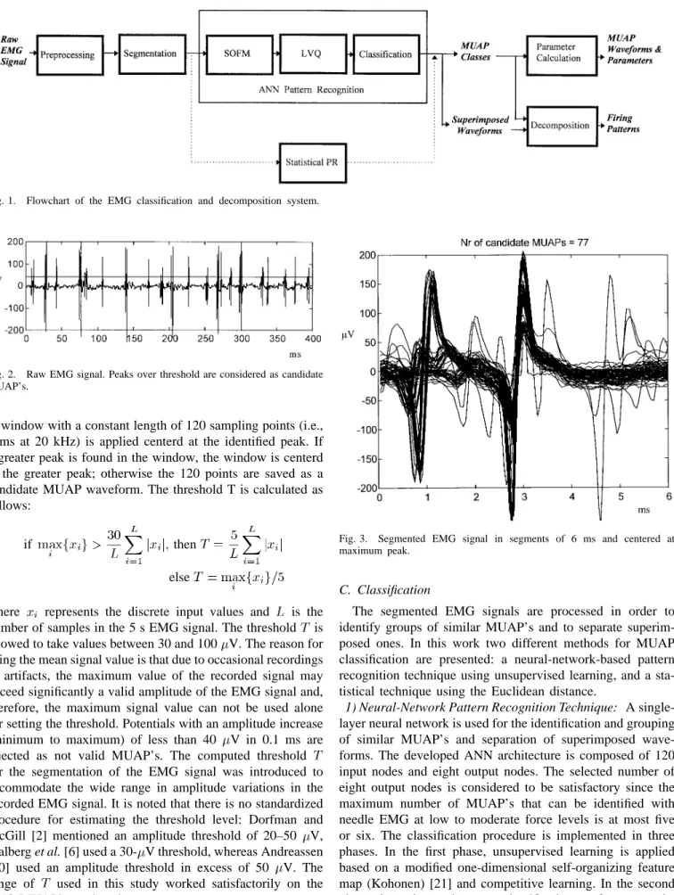
The proposed system consists of the following modules: i) data acquisition and preprocessing, ii) segmentation, iii) classification, iv) decomposition of superimposed waveforms, and v) parameter measurement. Fig. 1 illustrates the system flowchart.
A. Data Acquisition and Preprocessing
The EMG signal was recorded from the biceps brachii muscle at low to moderate force levels up to 30% of maximum voluntary contraction (MVC) under isometric conditions. The signal was acquired for 5 s, using the concentric needle electrode. The signal was analogue bandpass filtered at 3–10 kHz, and sampled at 20 kHz with 12-b resolution. The EMG signal was then low-pass filtered at 8 kHz.
B. Segmentation
The next step is to cut the EMG signal into segments of possible MUAP waveforms and eliminate areas of low activity. The segmentation algorithm calculates a threshold depending on the maximum value and the mean absolute value of the whole EMG signal. Peaks over the calculated threshold are considered as candidate MUAP’s.
Fig. 1. Flowchart of the EMG classification and decomposition system.
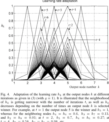
Fig. 2. Raw EMG signal. Peaks over threshold are considered as candidate MUAP’s.
A window with a constant length of 120 sampling points (i.e., 6 ms at 20 kHz) is applied centerd at the identified peak. If a greater peak is found in the window, the window is centerd at the greater peak; otherwise the 120 points are saved as a candidate MUAP waveform. The threshold T is calculated as follows:
if then
else
where represents the discrete input values and is the number of samples in the 5 s EMG signal. The threshold is allowed to take values between 30 and 100 V. The reason for using the mean signal value is that due to occasional recordings of artifacts, the maximum value of the recorded signal may exceed significantly a valid amplitude of the EMG signal and, therefore, the maximum signal value can not be used alone for setting the threshold. Potentials with an amplitude increase (minimum to maximum) of less than 40 V in 0.1 ms are rejected as not valid MUAP’s. The computed threshold for the segmentation of the EMG signal was introduced to accommodate the wide range in amplitude variations in the recorded EMG signal. It is noted that there is no standardized procedure for estimating the threshold level: Dorfman and McGill [2] mentioned an amplitude threshold of 20–50 V, Stalberg et al. [6] used a 30- V threshold, whereas Andreassen [10] used an amplitude threshold in excess of 50 V. The range of used in this study worked satisfactorily on the 1213 MUAP’s analyzed.
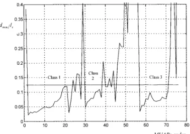
A typical EMG recording is given in Fig. 2, and the segmented signal waveforms are shown in Fig. 3.
Fig. 3. Segmented EMG signal in segments of 6 ms and centered at maximum peak.
C. Classification
The segmented EMG signals are processed in order to identify groups of similar MUAP’s and to separate superim-posed ones. In this work two different methods for MUAP classification are presented: a neural-network-based pattern recognition technique using unsupervised learning, and a sta-tistical technique using the Euclidean distance.
1) Neural-Network Pattern Recognition Technique: A single-layer neural network is used for the identification and grouping of similar MUAP’s and separation of superimposed wave-forms. The developed ANN architecture is composed of 120 input nodes and eight output nodes. The selected number of eight output nodes is considered to be satisfactory since the maximum number of MUAP’s that can be identified with needle EMG at low to moderate force levels is at most five or six. The classification procedure is implemented in three phases. In the first phase, unsupervised learning is applied based on a modified one-dimensional self-organizing feature map (Kohonen) [21] and competitive learning. In the second phase, in order to improve classification performance, the learning vector quantization method (LVQ2 by Kohonen) [21], is applied in a (self) supervised learning manner. In the third
such initialization may give different results at different runs. This is undesired when trying to evaluate and optimize the performance of the algorithm or when the physician wants to review the classification results. In order to avoid this problem, the weights of the output nodes are not initialized at small random values but at 0.0001, except for the weights of the fifth output node which are initialized at 0.01 times the amplitude values of the first segmented input. This leads to the result that at the first iteration, the fifth output node is always the winner since the distance d calculated as described in Step 2 has the smallest value. Thus, the classification results are always the same and the classes are assigned to the same output nodes for different runs. The fifth node was selected since it is in the middle of the output nodes in order to preserve the idea of the neighborhood. The implementation steps are as follows.
Step 1: Initialize weights at 0.0001, except the weights of the fifth output node which are initialized at values equal to 0.01 times the values of the first segmented input.
Step 2: Calculate distances between the input vector and weight vectors for each output node
where and
(1) The output node with minimum distance is the winner. Step 3: Adapt the weights. The weights for each output node and for each are adapted with
(2) The learning rate is a Gaussian function that gets narrower with the number of iterations , which means that the adaptation of the nodes neighboring to the winner decreases. The learning rate is also frequency sensitive for each output neuron, which means that it gets smaller the more often a neuron is selected as a winner
(3)
where is the winner node, is the number of
iterations, and is the number of times the specific node is selected as the winner. Setting the initial value of forces the network to fast learning even with a limited amount of data. When an output node is selected winner for the first time (i.e., a new class is identified), the factor and the learning
rate for If the calculated , then the
Fig. 4. Adaptation of the learning ratehkat the output nodesk at different iterations as given in (3) (withg = 1). It is illustrated that the neighborhood of hk is getting narrower with the number of iterations t, as well as hk decreases depending on the number of times an output node k is selected winner. For example, att = 1 the output node 5 is the winner and h5= 1, whereas for the neighboring nodes h4 = h6 = 0:6; h3 = h7 = 0:13;
and h2 = h8 = 0:01; at t = 2; h5 = 0:7; h4 = h6 = 0:27; at
t = 4; h5= 0:58; h4 = h6= 0:08; etc.
weights of the specific node are not adapted, since the change in the weights vector will be minimal. This is implemented in order to save computation time.
Step 4: Go to Step 2 and repeat for all segmented inputs. After all inputs are presented to the network, the first adaptation of the weights vector is completed and the system proceeds to the second learning phase. Fig. 4 illustrates the adaptation of the learning rate at the output nodes at different iterations as given in (3) (with . It is illustrated that the neighborhood of is getting narrower as the number of iterations increases. The learning rate gets its higher value for the winning node , whereas it gets significantly smaller values for the rest of the output nodes in the neighborhood. At the same time, decreases depending on the number of times an output node is selected winner.
b) Learning vector quantization (LVQ)—Learning phase 2: The task of this phase is to adapt the weights vectors slightly (move Voronoi vectors) in order to improve the classification performance [19], [21]. LVQ is actually a supervised learning technique, i.e., it demands forehand knowledge of correctly labeled (classified) inputs. Since such knowledge is not available, it is assumed that the adaptation carried out during the first learning phase is correct and, thus, the segmented inputs will be correctly classified. Weight adaptation and winner selection is again on-going as described in learning phase 1. In this modified version of LVQ2 the implementation steps are:
Step 1: Use the values of the weight vectors as obtained from learning phase 1.
Step 2: Present input and calculate distances between the input vector and weight vectors for each output node
Fig. 5. MUAP’s with similar shapes classified into three different classes.
is the first winner and the output node with the following minimum distance is the second winner .
Step 3: Adapt weights. The weights for the first winner output node are adapted with
(4) and for the second winner with
(5) The learning rate is initialized to 0.2 and decreases linearly with the number of times the specific node is selected as the first winner
(6)
If , then .
In other words, the weight vector with the correct label (first winner) is moved toward the input vector while the weight vector with the incorrect label (second winner) is moved away from it. The factor is used for controlling the adaptation of the second winner; if the input vector is close to the decision boundaries defined by the two winners, the factor takes a greater value moving the second winner far away from the input vector ; otherwise the adaptation is smaller.
Step 4: Go to Step 2 and repeat for all segmented inputs. After all inputs are presented to the network, the network is trained and the actual classification process starts.
c) Classification phase: In this phase all the input vectors will be classified to one of the output nodes and the superim-posed waveforms will be separated. The implementation steps are the following:
Step 1: Calculate distances between the input vector and the weight vectors as in (1). The output node with the minimum distance is the winner.
Step 2: In order to separate the superimposed waveforms from simple, nonoverlapping MUAP waveforms, the length of the weight vector of the winner node is calculated as the sum of the squares of its vector values
(7)
If then the input is assigned to the MUAP
class of the winner node else, the input is considered as a
superimposed waveform
The physical meaning of is that the greater its value the greater the dissimilarity between the waveforms.
Step 3: Go to Step 2 and repeat for all segmented inputs. Step 4: If the number of members in a class is three or more, the averaged MUAP waveform is computed and a valid MUAP class is identified; otherwise, the MUAP waveforms are saved with the superimposed waveforms for decomposition.
Fig. 5 illustrates the classification results of the segmented EMG signal given in Fig. 3 where MUAP’s with similar shapes are classified into three different classes.
2) Statistical Pattern Recognition Technique: In this itera-tive procedure the Euclidean distance is used in order to identify and group similar waveforms using a constant thresh-old. The implementation steps are the following:
Step 1: Start with the first waveform as input, being the first member of the class.
Step 2: Calculate the vector length of the input waveform and the distance between and all the other segmented waveforms as
where (8)
and
(9)
Step 3: Find the waveform with the minimum distance which is the one with the greatest similarity with and remove it from the input data set.
Step 4: Sliding and baseline correction. First slide the waveform with minimum distance up to two points backward and up to two points forward in order to find the best alignment position. Recalculate the distance for each case and assign the smallest as . Then, using the beginning and the ending parts of the MUAP waveforms, calculate baseline correction
as
(10)
Subtract from waveform and recalculate distance with . If it is smaller than , assign it as the new .
assign waveform to input ; go to Step 2
If the minimum distance divided by the vector length of the first waveform is less than a constant threshold, set to 0.125, then the two waveforms form a class. Then the class average is calculated and the procedure is repeated (go to Step 2 with the class average as input) comparing the class average now with all the rest waveforms in order to find the next waveform with the minimum distance. If the condition above is satisfied, then a new waveform is added to the class and a new class average is calculated, and so on. If not, the process stops; if the class members are more than or equal to three, then a MUAP class is formed and its averaged waveform is saved. If they are less than three, they are considered as superimposed waveforms. The process continues where it stopped comparing the last encountered waveform with all the remaining ones until all waveforms are processed. The baseline correction was applied selectively only to the waveform with the greatest similarity to the reference waveform and it was applied only if the distance between and with baseline correction was smaller than the distance without baseline correction. The use of baseline and slide correction improved the performance of the statistical pattern recognition technique by 5% as documented in Section III. Threshold values were chosen heuristically after extensive testing. It is noted that again there are no widely applicable threshold criteria for assigning a MUAP to a class. The value of 0.125 used in Step 5 was also used by Andreassen [10]. This threshold is critical because a smaller value may split a MUAP class with high waveform variability in two or more subclasses, whereas a greater threshold value may merge resembling MUAP classes. The averaged class waveforms are again the unique MUAP waveforms composing the EMG signal. Fig. 6 illustrates how the segmented signal waveforms of Fig. 3 are ordered according to their similarity
and how classes are formed where . The
MUAP classes are similar to the classes formed by the ANN pattern recognition technique in Fig. 5.
D. Decomposition of Superimposed Waveforms
The needle EMG signal recorded even at low to moderate force levels, contains superimposed potentials. It is important for correct firing rate analysis to identify as many MUAP’s as possible through decomposition of the superimposed wave-forms into their constituent MUAP’s. Although many studies have been published tackling the problem of EMG signal decomposition [3], [4], [7], [9], [12], [13], [16]–[18], no one
Fig. 6. MUAP waveforms ordered according to their similarity. MUAP’s withdmin=lx< 0:125 are grouped together into three different classes.
has gained wider acceptance outside the laboratory of origin and there are no standardized criteria for performing decompo-sition analysis. In this study, a simple decompodecompo-sition procedure is introduced, where the decomposition algorithm is based on the crosscorrelation of the unique MUAP waveforms with the superimposed waveforms. It is assumed that the correct unique MUAP waveforms composing the superimposed ones are known through one of the previous classification processes. The Euclidean distance and area measures are combined in a heuristic way for decomposing the superimposed waveforms. The decomposition steps are as follows.
Step 1: For each unique MUAP waveform, extract the main part of the MUAP that contains the main spike as follows: Reduce the unique MUAP lengths by dropping the beginning and ending parts of the waveform that are less than 1/15 of the MUAP amplitude (minimum to maximum). The 1/15 of the MUAP amplitude is an estimate of the beginning and ending points of the MUAP main spike. This is critical in order to crosscorrelate only the most important part of the MUAP.
Step 2: Select a superimposed waveform .
Step 3: Crosscorrelate each reduced MUAP with the super-imposed waveform and find the best matching point, i.e., the point where the crosscorrelation coefficient takes its maximum value.
Step 4: For each matching pair calculate the normalized Euclidean distance, the area difference, and a varying thresh-old. The normalized Euclidean distance is the sum of squares of the values obtained by the subtraction of the reduced MUAP waveform c from the superimposed waveform for the reduced MUAP length , divided by the sum of squares of the reduced MUAP vector values
(11)
The average area difference is the average of the absolute values obtained by the subtraction of the reduced MUAP from the superimposed waveform for the reduced
(a) (b) (c)
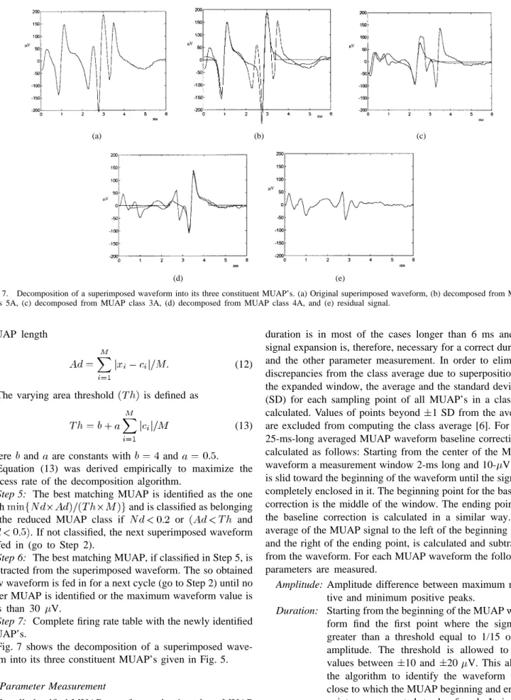
(d) (e)
Fig. 7. Decomposition of a superimposed waveform into its three constituent MUAP’s. (a) Original superimposed waveform, (b) decomposed from MUAP class 5A, (c) decomposed from MUAP class 3A, (d) decomposed from MUAP class 4A, and (e) residual signal.
MUAP length
(12)
The varying area threshold is defined as
(13)
where and are constants with and
Equation (13) was derived empirically to maximize the success rate of the decomposition algorithm.
Step 5: The best matching MUAP is identified as the one
with and is classified as belonging
to the reduced MUAP class if or and
. If not classified, the next superimposed waveform is fed in (go to Step 2).
Step 6: The best matching MUAP, if classified in Step 5, is subtracted from the superimposed waveform. The so obtained new waveform is fed in for a next cycle (go to Step 2) until no other MUAP is identified or the maximum waveform value is less than 30 V.
Step 7: Complete firing rate table with the newly identified MUAP’s.
Fig. 7 shows the decomposition of a superimposed wave-form into its three constituent MUAP’s given in Fig. 5. E. Parameter Measurement
For all classified MUAP waveforms, the 6-ms-long MUAP segments are expanded to 25 ms on the original EMG sig-nal where the position of the identified MUAP peak was marked during segmentation. The rationale is that the MUAP
duration is in most of the cases longer than 6 ms and the signal expansion is, therefore, necessary for a correct duration and the other parameter measurement. In order to eliminate discrepancies from the class average due to superpositions in the expanded window, the average and the standard deviation (SD) for each sampling point of all MUAP’s in a class are calculated. Values of points beyond 1 SD from the average are excluded from computing the class average [6]. For each 25-ms-long averaged MUAP waveform baseline correction is calculated as follows: Starting from the center of the MUAP waveform a measurement window 2-ms long and 10- V high is slid toward the beginning of the waveform until the signal is completely enclosed in it. The beginning point for the baseline correction is the middle of the window. The ending point for the baseline correction is calculated in a similar way. The average of the MUAP signal to the left of the beginning point and the right of the ending point, is calculated and subtracted from the waveform. For each MUAP waveform the following parameters are measured.
Amplitude: Amplitude difference between maximum nega-tive and minimum posinega-tive peaks.
Duration: Starting from the beginning of the MUAP wave-form find the first point where the signal is greater than a threshold equal to 1/15 of the amplitude. The threshold is allowed to take values between 10 and 20 V. This allows the algorithm to identify the waveform areas close to which the MUAP beginning and ending points are expected to be found. It is also noted that threshold values in this range were used by Stalberg et al. [1]. Starting from that point and moving backward to the beginning
Fig. 8. Average MUAP waveforms expanded to 25 ms with the calculated parameters.
of the waveform, a measurement window 1 ms long and 10 V high is slid until the signal is completely enclosed in it. The point in the window closer to the baseline is the MUAP beginning point. The MUAP ending point is calculated in a similar way. The duration of the MUAP is the time interval between MUAP beginning and ending points.
Area: Rectified MUAP integrated over the calculated duration.
Rise Time: Time between maximum negative peak and the preceding minimum positive peak within the duration.
Phases: Number of baseline crossings within the dura-tion where amplitude exceeds 25 V, plus one.
Turns: Number of positive and negative peaks where the differences from the preceding and follow-ing turn exceed 25 V.
Fig. 8 displays the expanded MUAP waveforms of Fig. 5 with the calculated parameters.
III. RESULTS
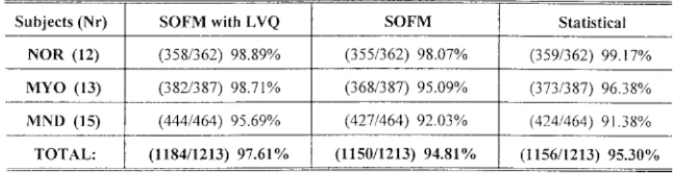
EMG data collected from 40 subjects were analyzed using the pattern recognition techniques described in Section II. Data were recorded from 12 normal (NOR) subjects, 13 subjects suffering from myopathy (MYO) and 15 subjects suffering from motor neuron disease (MND). Diagnostic criteria were based on clinical opinion, biochemical data and muscle biopsy.
Only subjects with no history or signs of neuromuscular disorders were considered as normal. Table I shows the clas-sification success rate on 1213 MUAP’s, obtained from 576 EMG recordings. The classification success rate was defined as the percentage ratio of the correctly identified MUAP classes by the algorithm and the number of true MUAP classes present in the signal as identified by an experienced neurophysiologist. The average success rate for the SOFM with LVQ algorithm was 97.6%, for the SOFM algorithm alone 94.8%, and for the statistical pattern recognition algorithm 95.3%. The ANN technique also yielded good results without the LVQ learning phase. Examining the classification success rate for each class, the highest success rate was obtained for the NOR group and the lowest for the MND group. This was the case for all three algorithms. The lowest success rate for the MND group is attributed to the more complex and variable waveform shapes. Also, as shown in Table I, the SOFM with LVQ algorithm improved significantly the success rate for the MND group compared to the other two algorithms. The statistical algorithm gave the highest success rate for the NOR group and the lowest for the MND group compared to the other two algorithms. The use of slide and baseline correction in the statistical technique improved the classification success rate by about 5%. In general, where all three algorithms failed to identify a MUAP class, it was because of inadequate number of class members in the signal and due to waveform variability. In some rare cases MUAP classes with very similar shapes were grouped together. Downsampling the signal by a factor of two at 10 kHz, saved computation time but reduced the success rate by about 1.5% in all cases. The very small reduction in the success rate, is attributed to the fact that approximately 95% of the power content of the whole population of MUAP’s investigated falls below 2500 Hz [24]. Thus, downsampling the EMG signal by two, it minimally affects the information content of the signal.
For the decomposition of the superimposed waveforms, the algorithm correctly identified about 90% of the MUAP occurrences in the superimposed waveforms. Fig. 7 illustrates an example where a superimposed waveform composed of three different MUAP’s was successfully decomposed.
MATLAB was used for implementing the above algorithms. The processing time on a PC Pentium 233 MHz for a 5-s epoch EMG signal with 77 waveforms was about 0.5 s for the segmentation and about 0.6 s for the classification with SOFM with LVQ, 0.4 s for SOFM, and 1 s for the statistical technique. The processing time for the decomposition of each superim-posed waveform with three classes was about 0.02 s. Since
MATLAB is an interpreter, all the timings may be significantly improved by the use of a compiled version of the algorithms.
IV. DISCUSSION
The decomposition of real EMG signals into their con-stituent MUAP’s and their classification into groups of similar shapes is a typical case of an unsupervised learning pattern recognition problem. The number of MUAP classes composing the EMG signal, the number of MUAP’s per class, their firing pattern, and the expected shape of the MUAP waveforms are unknown. The problem gets even more difficult because of MUAP waveform variability, jitter of single fiber potentials, and MUAP superpositions. Any automated method for EMG analysis should require no operator intervention; should be fast, robust and reliable; and achieve high success rate in order to be of clinical use. Most of the previous methods briefly described in Section I used mainly template matching which requires a predetermination of the classification boundaries and may fail to detect classes with insufficient frequency of MUAP repetitions and MUAP’s with high shape variability. Also, the need for operator intervention, especially in some of the earlier works on the topic [3], [4], and long processing time make their applicability in routine clinical environment difficult, although a high success rate has been reported.
In this work, two different pattern recognition techniques for the classification of MUAP’s were investigated: i) an artificial neural network technique based on unsupervised learning, using modified SOFM and LVQ, and ii) a statistical pattern recognition technique based on the Euclidean distance. Both pattern recognition techniques described are quite simple in their concepts, and gave a high success rate. The ANN tech-nique performed better than the statistical pattern recognition technique and yielded a higher success rate. ANN’s seem more appropriate for the classification of MUAP’s because of their ability to adapt and to create complex classification boundaries. The additional use of the LVQ algorithm with the SOFM algorithm optimizes the classification boundaries through slight adaptation of the weights vectors. The result of this process is twofold: i) MUAP’s with high variability which during the first learning phase were sorted out as superimposed, to be moved into the MUAP waveform classes, and ii) multiple classes of the same MUAP to be merged. The improvement of the classification performance is clearly demonstrated in the case of the MND group which contains MUAP’s with more complex and variable waveform shapes, where the classification success rate of the SOFM with the LVQ algorithm was considerably higher compared to the statistical one. The combination of SOFM with LVQ for fine tuning of the network was also used successfully in speech recognition [21]. Moreover, the ANN technique presented in this study performed well even with a limited amount of data and achieved fast learning in only one epoch. Standard SOFM and standard competitive learning algorithms, investigated for the same real data, required a much greater number of learning epochs in order to converge. The difference between the SOFM algorithm implemented in this study and the standard SOFM [21] is that in the standard SOFM the learning rate is
not frequency sensitive, whereas in competitive learning only the first winner is adapted (winner takes it all). The “pseudoun-supervised” learning algorithm as proposed by Hassoun et al. [17], [18] has a complicated network architecture, requires many learning epochs, and is computationally demanding.
The statistical technique utilized in this study has the disadvantage of using a constant threshold for classification that makes it less flexible, especially when the signal is noisy and with high variability. This has as a result that during the classification phase less MUAP occurrences are identified in comparison to the ANN technique. Also, the computational time increases geometrically with the amount of processed data. On the other hand, the number of classes which can be detected by the statistical technique is unlimited depending only on the number of actual MUAP classes existing in the signal. A similar approach was used by Loudon et al. [16], with the difference that waveforms were compared with the last encountered waveform instead of the group average which may lead to less accurate classification results.
It was also observed in both techniques that often, due to waveform variability, MUAP classes coming from the same motor unit, although they looked similar, were not grouped together. Merging of these classes can be achieved by: i) using the firing statistics after the decomposition process or ii) using the statistical pattern recognition technique in a second iteration with a greater constant threshold 0.3) and the averaged class waveforms as input.
Another concern is the selection of the length of the segmentation window. In this work the 6-ms-long window was chosen as covering the main MUAP spike duration in most of the disease cases. A shorter window would fail to contain the main MUAP spike in the case of motor neuron disease where MUAP’s usually have a much longer duration. This would cause the classification algorithms to fail or would cut a long polyphasic MUAP into two artificial potentials. On the other hand, a shorter segmentation window would result in the identification of more potential occurrences during the classification process in the case of normal or myopathic signals, since only the main spike would be included. The decomposition of the superimposed waveforms complements this drawback in this work.
The time domain vector of the segmented signal was used as input to the classification algorithms without any normal-ization. This proved to give better results than the frequency domain vector [25] or the use of features characterizing the signal. This is due to the relatively simple shapes of the MUAP waveforms as these may still be identified at low to moderate force levels. Furthermore, the results in this study can be compared with a parametric pattern recognition algorithm where MUAP parameters were input to the classifier [14], [15] and which was evaluated with the same data set. The classification performance was poorer but the algorithm was computationally more efficient since the dimension of the input vector was significantly reduced.
Several new ideas were introduced in this work in order to improve the performance of the algorithms.
1) Learning achieved in only one epoch in the SOFM and LVQ algorithms.
4) The threshold in the classification phase of the ANN technique in order to separate the superimposed wave-forms.
5) The combination of Euclidean distance and area mea-sures in the decomposition of the superimposed wave-forms in order to classify the decomposed wavewave-forms. In conclusion, the pattern recognition techniques as de-scribed in this work make possible the development of a fully automated EMG signal analysis system which is accurate, simple, fast, and reliable enough to be used in routine clin-ical environment. Future work will evaluate the algorithms developed in this study on EMG data recorded from more muscles and more subjects. In addition, this system may be integrated into a hybrid diagnostic system for neuromuscular diseases based on ANN where EMG [15], muscle biopsy, biochemical and molecular genetic findings, and clinical data may be combined to provide a diagnosis [26].
REFERENCES
[1] E. Stalberg, S. Andreassen, B. Falck, H. Lang, A. Rosenfalck, and W. Trojaborg, “Quantitative analysis of individual motor unit potentials: A proposition for standardized terminology and criteria for measurement,”
J. Clin. Neurophysiol., vol. 3, no. 4, pp. 313–348, 1986.
[2] L. J. Dorfman and K. C. McGill, “AAEE minimonograph #29: Auto-matic quantitative electromyography,” Muscle and Nerve, vol. 11, pp. 804–818, 1988.
[3] R. S. LeFever and C. J. DeLuca, “A procedure for decomposing the myoelectric signal into its constituent action potentials: I. Technique, theory and implementation,” IEEE Trans. Biomed. Eng., vol. BME-29, pp. 149–157, Mar. 1982.
[4] , “A procedure for decomposing the myoelectric signal into its constituent action potentials: II. Execution and test for accuracy,” IEEE
Trans. Biomed. Eng., vol. BME-29, pp. 158–164, Mar. 1982.
[5] E. Stalberg and L. Antoni, “Computer aided EMG analysis,” in
Computer-Aided Electromyography and Expert Systems, vol. 10, J.
E. Desmedt, Ed. Amsterdam, the Netherlands: Elsevier Science, 1983, pp. 186–234.
[6] E. Stalberg, B. Falck, M. Sonoo, S. Stalberg, and M. Astrom, “Multi-MUP EMG analysis—A two year experience in daily clinical work,”
Electroencelography and Clinical Neurophysiology 97. Amsterdam, the Netherlands: Elsevier Science, 1995, pp. 145–154.
[7] P. Guihenec, J. Calamel, C. Doncarli, D. Gitton, and C. Michel, “Automatic detection and pattern recognition of signal motor unit po-tentials in needle EMG,” Computer-Aided Electromyography—Progress
in Clinical Neurophysiology, vol. 10, J. E. Desmedt, Ed. Amsterdam, the Netherlands: Elsevier Science, 1983, pp. 73–127.
[8] J. L. Coatrieux, P. Toulouse, B. Rouvrais, and R. Le Bars, “Automatic classification of electromyographic signals,” EEG Clin. Neurophysiol., vol. 55, pp. 333–341, 1983.
[9] K. C. McGill, K. L. Cummins, and L. J. Dorfman, “Automatic decom-position of the clinical electromyogram,” IEEE Trans. Biomed. Eng., vol. BME-32, pp. 470–477, July 1985.
[10] S. Andreassen, “Methods for computer-aided measurement of motor unit parameters,” in Proc. The London Symp., R. J. Ellington et al., Eds., 1987, EEG suppl. 39, pp. 13–20.
[16] G. H. Loudon, N. B. Jones, and A. S. Sehmi, “New signal processing techniques for the decomposition of EMG signals,” Med. Biol. Eng.
Comput., Nov. 1992, pp. 591–599.
[17] M. H. Hassoun, C. Wang, and A. R. Spitzer, “NNERVE: Neural network extraction of repetitive vectors for electromyography—Part I: Algorithm,” IEEE Trans. Biomed. Eng., vol. 41, pp. 1039–1052, Nov. 1994.
[18] , “NNERVE: Neural network extraction of repetitive vectors for electromyography—Part II: Performance analysis,” IEEE Trans.
Biomed. Eng., vol. 41, pp. 1053–1061, Nov. 1994.
[19] S. Haykin, Neural Networks—A Comprehensive Foundation. New York: Macmillan College., 1994.
[20] B. Kroesse and P. Van der Smagt, An Introduction to Neural Networks. Amsterdam, the Netherlands: Univ. Amsterdam Press, 1993.
[21] T. Kohonen, “The self-organizing map,” Proc. IEEE, vol. 78, pp. 1464–1480, Sept. 1990.
[22] C. I. Christodoulou and C. S. Pattichis, “A new technique for the classification and decomposition of EMG signals,” in Proc. IEEE Int.
Conference on. Neural Networks, Perth, Western Australia, Nov. 1995,
vol. 5, pp. 2303–2308.
[23] R. P. Lippmann, “An introduction to computing with neural nets,” IEEE
Acoust., Speech, Signal Processing, Mag., vol. 4, pp. 4–22, Apr. 1987.
[24] C. S. Pattichis, M. S. Pattichis, and C. N. Schizas, “MUAP wavelet analysis,” in Proc. Annu. Int. Conf. IEEE Eng. Medicine and Biology
Society, Amsterdam, Netherlands, 1996, vol. 18, paper no. 553.
[25] D. Stashuk and R. Naphan, “Classification performance of different motor unit action potential feature space representations: A simulation study,” in Proc. Annu. Int. Conf. IEEE Eng. Medicine and Biology
Society, 1990, vol. 12, no. 5, pp. 2225–2226
[26] C. N. Schizas, C. S. Pattichis, and C. A. Bonsett, “Medical diagnostic systems: A case for neural networks,” Technol., Health Care, vol. 2, pp. 1–18, 1994.
Christodoulos I. Christodoulou was born in Paphos, Cyprus, in 1961. He received the diploma in electrical engineering with specialization in telecommunications from the Technical University of Aachen, Germany, in 1987. He is currently working toward the Ph.D. degree in electronic engineering at the Queen Mary and Westfield College, University of London, London, U.K.
Since 1990, he is employed as a Programmer Analyst in the Information Technology department of the Cyprus Popular Bank, Cyprus. He carries out his research work in cooperation with the Cyprus Institute of Neurology and Genetics and the department of Computer Science of the University of Cyprus. His research interests include neural networks, pattern recognition, image and signal processing, and their applications in biomedicine.
Constantinos S. Pattichis (S’83–M’88) was born in Nicosia, Cyprus, on January 30, 1959. He received the M.Sc. degree in biomedical engineering from the University of Texas at Austin, in 1984 and the Ph.D. degree in electronic engineering from the University of London, London, U.K., in 1992. He is currently an Assistant Professor with the Department of Computer Science at the University of Cyprus, Cyprus. His current research interests include medical imaging, biosignal analysis, health telematics, intelligent systems, artificial neural networks, and genetic algorithms.