Politecnico di Torino
Porto Institutional Repository
[Article] Infrequent Weighted Itemset Mining Using Frequent Pattern Growth
Original Citation:
Cagliero L.; Garza P. (2014).
Infrequent Weighted Itemset Mining Using Frequent Pattern Growth.
In:
IEEE TRANSACTIONS ON KNOWLEDGE AND DATA ENGINEERING
, vol. 26 n. 4, pp.
903-915. - ISSN 1041-4347
Availability:
This version is available at :
http://porto.polito.it/2514489/
since: September 2013
Publisher:
IEEE COMPUTER SOCIETY
Published version:
DOI:
10.1109/TKDE.2013.69
Terms of use:
This article is made available under terms and conditions applicable to Open Access Policy Article
("Public - All rights reserved") , as described at
http://porto.polito.it/terms_and_conditions.
html
Porto, the institutional repository of the Politecnico di Torino, is provided by the University Library
and the IT-Services. The aim is to enable open access to all the world. Please
share with us
how
this access benefits you. Your story matters.
Infrequent Weighted Itemset Mining
using Frequent Pattern Growth
Luca Cagliero and Paolo Garza
Abstract
Frequent weighted itemsets represent correlations frequently holding in data in which items may weight differently. However, in some contexts, e.g., when the need is to minimize a certain cost function, discovering rare data correlations is more interesting than mining frequent ones. This paper tackles the issue of discovering rare and weighted itemsets, i.e., the Infrequent Weighted Itemset (IWI) mining problem. Two novel quality measures are proposed to drive the IWI mining process. Furthermore, two algorithms that perform IWI and Minimal IWI mining efficiently, driven by the proposed measures, are presented. Experimental results show efficiency and effectiveness of the proposed approach.
Index Terms
H.2.8.b Clustering, classification, and association rules, H.2.8.d Data mining
I. INTRODUCTION
Itemset mining is an exploratory data mining technique widely used for discovering valuable correlations among data. The first attempt to perform itemset mining [1] was focused on discovering frequent itemsets, i.e., patterns whose observed frequency of occurrence in the source data (the support) is above a given threshold. Frequent itemsets find application in a number of real-life contexts (e.g., market basket analysis [1], medical image process-ing [2], biological data analysis [3]). However, many traditional approaches ignore the influence/interest of each item/transaction within the analyzed data. To allow treating items/transactions differently based on their relevance in the frequent itemset mining process, the notion of weighted itemset has also been introduced [4]–[6]. A weight is associated with each data item and characterizes its local significance within each transaction.
Consider, as an example, the dataset reported in Table I. It includes 6 transactions (identified by the respective
tids), each one composed of 4 distinct items weighted by the corresponding degree of interest (e.g., item a has
weight 0 in tid 1, and 100 in tid 4). In the contexts of data center resource management and application profiling, transactions may represent CPU usage readings collected at a fixed sampling rate. For instance, tid 1 means that, at
a fixed point of time (1), CPUbworks at a high usage rate (weight 100), CPUscanddhave an intermediate usage
rate (weights 57 and 71, respectively), while CPU ais temporarily idle (weight 0). The itemsets mined from the
L. Cagliero and P. Garza are with the Dipartimento di Automatica e Informatica, Politecnico di Torino, Corso Duca degli Abruzzi 24, 10129, Torino, Italy. E-mail:{luca.cagliero, paolo.garza}@polito.it.
TABLE I
EXAMPLE OF WEIGHTED TRANSACTIONAL DATASET
Tid CPU usage readings
1 ⟨a,0⟩ ⟨b,100⟩ ⟨c,57⟩ ⟨d,71⟩ 2 ⟨a,0⟩ ⟨b,43⟩ ⟨c,29⟩ ⟨d,71⟩ 3 ⟨a,43⟩ ⟨b,0⟩ ⟨c,43⟩ ⟨d,43⟩ 4 ⟨a,100⟩ ⟨b,0⟩ ⟨c,43⟩ ⟨d,100⟩ 5 ⟨a,86⟩ ⟨b,71⟩ ⟨c,0⟩ ⟨d,71⟩ 6 ⟨a,57⟩ ⟨b,71⟩ ⟨c,0⟩ ⟨d,71⟩ TABLE II
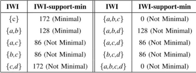
IWIS EXTRACTED FROM THE DATASET INTABLEI. MAXIMUMIWI-SUPPORT-MIN THRESHOLDξ=180.
IWI IWI-support-min IWI IWI-support-min
{c} 172 (Minimal) {a,b,c} 0 (Not Minimal)
{a,b} 128 (Minimal) {a,b,d} 128 (Not Minimal)
{a,c} 86 (Not Minimal) {a,c,d} 86 (Not Minimal)
{b,c} 86 (Not Minimal) {b,c,d} 86 (Not Minimal)
{c,d} 172 (Not Minimal) {a,b,c,d} 0 (Not Minimal) TABLE III
IWIS EXTRACTED FROM THE DATASET INTABLEI. MAXIMUMIWI-SUPPORT-MAX THRESHOLDξ=390.
IWI IWI-support-max IWI IWI-support-max
{a} 286 (Minimal) {a,c} 372 (Not Minimal)
{b} 285 (Minimal) {b,c} 371 (Not Minimal)
{c} 172 (Minimal)
example dataset can be exploited by a domain expert to profile system usage in order to perform resource allocation and system resizing.
The significance of a weighted transaction, i.e., a set of weighted items, is commonly evaluated in terms of the corresponding item weights. Furthermore, the main itemset quality measures (e.g., the support) have also been tailored to weighted data and used for driving the frequent weighted itemset mining process. For instance, when
evaluating the support of {a,b} in the example dataset reported in Table I, the occurrence of b in tid 1, which
represents a highly utilized CPU, should be treated differently from the one ofa, which represents an idle CPU at
the same instant. In [4]–[6] different approaches to incorporating item weights in the itemset support computation have been proposed. Note that they are all tailored to frequent itemset mining, while this work focuses on infrequent itemsets.
In recent years, the attention of the research community has also been focused on the infrequent itemset mining problem, i.e., discovering itemsets whose frequency of occurrence in the analyzed data is less than or equal to a maximum threshold. For instance, in [7], [8] algorithms for discoveringminimalinfrequent itemsets, i.e., infrequent
itemsets that do not contain any infrequent subset, have been proposed. Infrequent itemset discovery is applicable to data coming from different real-life application contexts such as (i) statistical disclosure risk assessment from census data and (ii) fraud detection [7]–[9]. However, traditional infrequent itemset mining algorithms still suffer from their inability to take local item interestingness into account during the mining phase. In fact, on the one hand, itemset quality measures used in [4]–[6] to drive the frequent weighted itemset mining process are not directly applicable to accomplish the infrequent weighted itemset mining task effectively, while, on the other hand, state-of-the-art infrequent itemset miners are, to the best of our knowledge, unable to cope with weighted data.
This paper addresses the discovery of infrequent and weighted itemsets, i.e., the Infrequent Weighted Itemsets (IWIs), from transactional weighted datasets. To address this issue, the IWI-support measure is defined as a weighted frequency of occurrence of an itemset in the analyzed data. Occurrence weights are derived from the weights associated with items in each transaction by applying a given cost function. In particular, we focus our attention on two different IWI-support measures: (i) The IWI-support-min measure, which relies on a minimum cost function, i.e., the occurrence of an itemset in a given transaction is weighted by the weight of itsleast interesting item, (ii) The IWI-support-max measure, which relies on a maximum cost function, i.e., the occurrence of an itemset in a
given transaction is weighted by the weight of themostinteresting item. Note that, when dealing with optimization
problems, minimum and maximum are the most commonly used cost functions. Hence, they are deemed suitable for driving the selection of a worthwhile subset of infrequent weighted data correlations. Specifically, the following problems have been addressed:
A) IWI and Minimal IWI mining driven by a maximum IWI-support-min threshold, and B) IWI and Minimal IWI mining driven by a maximum IWI-support-max threshold.
Task (A) entails discovering IWIs and Minimal IWIs (MIWIs) which include the item(s) with the least local interest within each transaction. Table II reports the IWIs mined from Table I by enforcing a maximum IWI-support-min
threshold equal to 180 and their corresponding IWI-support-min values. For instance,{a,b}covers the transactions
with tids 1, 2, 3, and 4 with a minimal weight 0 (associated withain tids 1 and 2 andb in tids 3 and 4), while it
covers the transactions with tids 5 and 6 with minimal weights 71 and 57, respectively. Hence, its IWI-support-min
value is 128. In the context of system usage profiling, IWIs in Table II represent sets of CPUs which containat
leastone underutilized or idle CPU at each sampled instant. As shown in Section V, real-life system malfunctioning
or underutilization may arise when the workload is not allocated properly over the available CPUs. For instance,
considering CPUsaandb, recognizing a suboptimal usage rate of at least one of them may trigger targeted actions,
such as system resizing or resource sharing policy optimization. As an extreme case,{a,b,c} has IWI-support-min
equal to 0 because at every sampled point of time at least one betweena,b, orc(not necessarily the same at each
instant) is idle, possibly due to system oversizing. Considering Minimal IWIs (MIWIs) allows the expert to focus
her/his attention on the smallest CPU sets that contain at least one underutilized/idle CPU and, thus, reduces the
bias due to the possible inclusion of highly weighted items in the extracted patterns. In Table II IWIs are partitioned between minimal and not, as indicated next to each itemset IWI-support-min value (Minimal/Not Minimal).
Task (B) entails discovering IWIs and MIWIs which include item(s) having maximal local interest within each transaction by exploiting the IWI-support-max measure. Table III reports the IWIs mined from Table I by enforcing
a maximum IWI-support-max threshold equal to 390. They may represent sets of CPUs which containonly
under-utilized/idle CPUs at each sampled time instant. Note that, in this context, discovering large CPU combinations may be deemed particularly useful by domain experts, because they represent large resource sets which could be reallocated.
To accomplish tasks (A) and (B), we present two novel algorithms, namely Infrequent Weighted Itemset Miner (IWI Miner) and Minimal Infrequent Weighted Itemset Miner (MIWI Miner), which perform IWI and MIWI mining driven by IWI-support thresholds. IWI Miner and MIWI Miner are FP-Growth-like mining algorithms [10], whose main features may be summarized as follows: (i) Early FP-tree node pruning driven by the maximum IWI-support constraint, i.e., early discarding of part of the search space thanks to a novel item pruning strategy, and (ii) cost function-independence, i.e., they work in the same way regardless of which constraint (either IWI-support-min or IWI-support-max) is applied, (iii) early stopping of the recursive FP-tree search in MIWI Miner to avoid extracting non-minimal IWIs. As shown in Section IV, Property (ii) makes tasks (A) and (B) equivalent, from an algorithmic point of view, as long as a preliminary data transformation step, which adapts data weights according to the selected aggregation function, is applied before accomplishing the mining task.
Experiments, performed on both synthetic and real-life datasets, show efficiency and effectiveness of the proposed approach. In particular, they show the characteristics and usefulness of the itemsets discovered from data coming from benchmarking and real-life multi-core systems, as well as the algorithm scalability.
This paper is organized as follows. Section II discusses and compares related work with the proposed approach. Section III introduces preliminary definitions and notations as well as formally states the IWI and MIWI mining tasks addressed by this paper. Section IV describes the proposed algorithms, while Section V evaluates efficiency and effectiveness of the proposed approach. Finally, Section VI draws conclusions and presents future work.
II. PREVIOUS WORK
Frequent itemset mining is a widely used data mining technique that has been introduced in [1]. In the traditional itemset mining problem items belonging to transactional data are treated equally. To allow differentiating items based on their interest or intensity within each transaction, in [4] the authors focus on discovering more informative association rules, i.e., the Weighted Association Rules (WAR), which include weights denoting item significance. However, weights are introduced only during the rule generation step after performing the traditional frequent itemset mining process. The first attempt to pushing item weights into the itemset mining process has been done in [5]. It proposes to exploit the anti-monotonicity of the proposed weighted support constraint to drive the Apriori-based itemset mining phase. However, in [4], [5] weights have to be preassigned, while, in many real-life cases, this might not be the case. To address this issue, in [6] the analyzed transactional dataset is represented as a bipartite hub-authority graph and evaluated by means of a well-known indexing strategy, i.e., HITS [11], in order to automate item weight assignment. Weighted item support and confidence quality indexes are defined accordingly and used
for driving the itemset and rule mining phases. This paper differs from the above-mentioned approaches because it focuses on mining infrequent itemsets from weighted data instead of frequent ones. Hence, different pruning techniques are exploited.
A related research issue is probabilistic frequent itemset mining [12], [13]. It entails mining frequent itemsets from uncertain data, in which item occurrences in each transaction are uncertain. To address this issue, probabilistic models have been constructed and integrated in Apriori-based [12] or projection-based [14] algorithms. Although probabilities of item occurrence may be remapped to weights, the semantics behind probabilistic and weighted itemset mining is radically different. In fact, the probability of occurrence of an item within a transaction may be totally uncorrelated with its relative importance. For instance, an item that is very likely to occur in a given transaction may be deemed the least relevant one by a domain expert. Furthermore, this paper differs from the above-mentioned approaches as it specifically addresses the infrequent itemset mining task.
A parallel effort has been devoted to discovering rare correlations among data, i.e., the infrequent itemset mining problem [7]–[9], [15]–[17]. For instance, in [7], [8] a recursive algorithm for discovering minimal unique itemsets from structured datasets, i.e., the shortest itemsets with absolute support value equal to 1, is proposed. They extend a preliminary algorithm version, previously proposed in [18], by specifically tackling algorithm scalability issues. The authors in [9] first addressed the issue of discovering minimal infrequent itemsets, i.e., the itemsets that satisfy a maximum support threshold and do not contain any infrequent subset, from transactional datasets. More recently, in [17] an FP-Growth-like algorithm for mining minimal infrequent itemsets has also been proposed. To reduce the computational time the authors introduce the concept of residual tree, i.e., an FP-tree associated with a generic
itemi that represents dataset transactions obtained by removing i. Similarly to [17], in this paper we propose an
FP-tree-based approach to mining infrequent itemsets. However, unlike all of the above-mentioned approaches, we face the issue of treating items differently, based on their relative importance in each transaction, in the discovery of infrequent itemsets from weighted data. Furthermore, unlike [17], we adopt a different item pruning strategy tailored to the traditional FP-tree structure to perform IWI mining efficiently. An attempt to exploit infrequent itemsets in mining positive and negative association rules has also been made in [15], [16]. Since infrequent itemset mining is considered an intermediate step, their focus is radically different from that of this paper.
III. PROBLEM STATEMENT
This paper addresses the problem of mining infrequent itemsets from transactional datasets. LetI={i1, i2,. . .,
im}be a set of data items. A transactional datasetT={t1,t2,. . .,tn}is a set of transactions, where each transaction
tq (q∈[1, n]) is a set of items inI and is characterized by a transaction ID (tid).
An itemset I is a set of data items [1]. More specifically, we denote as k-itemset a set of k items in I. The
support (or occurrence frequency) of an itemset is the number of transactions containing I in T. An itemset I
is infrequent if its support is less than or equal to a predefined maximum support threshold ξ. Otherwise, it is
said to be frequent [1]. An infrequent itemset is said to beminimalif none of its subsets is infrequent [7]. Given
entails discovering all infrequent (minimal) itemsets fromT [9].
Unfortunately, using the traditional support measure for driving the itemset mining process entails treating items and transactions equally, even if they do not have the same relevance in the analyzed dataset. To treat items differently within each transaction we introduce the concept of weighted item as a pair ⟨ik, w
q
k⟩, where ik ∈ I is an item contained intq ∈T, whilew
q
k is the weight associated withik that characterizes its local interest/intensity
in tq [4]. Concepts of weighted transaction and weighted transactional dataset are defined accordingly as sets of
weighted items and weighted transactions, respectively.
Definition 1: Weighted transactional dataset.LetI={i1,i2,. . .,im}be a set of items. A weighted transactional
datasetTwis a set of weighted transactions, where each weighted transactiontwq is a set of weighted items⟨ik, wqk⟩ such thatik ∈ I andwqk is the weight associated withik intwq.
Note that, in general, weights could be either positive, null, or negative numbers. Itemsets mined from weighted transactional datasets are calledweighted itemsets. Their expression is similar to the one used for traditional itemsets, i.e., a weighted itemset is a subset of the data items occurring in a weighted transactional dataset. The problem
of mining itemsets by considering weights associated with each item is known as the weighted itemset mining
problem [4]. For the sake of simplicity, by convenient abuse of notation weighted itemsets will be denoted by
itemsets whenever it is clear from the context. For the same reason, a generic weighted dataset and transaction are
denoted by T andtq, respectively, throughout the paper.
Consider again the example dataset reported in Table I. It is a weighted transactional dataset T composed of
6 transactions, each one including 4 weighted items. Since, for instance, the weight of item a in tid 1 (0) is
significantly lower than the ones of b (100) and d (71) thena, b, and dshould be treated differently during the
mining process.
This paper focuses on considering item weights in the discovery of infrequent itemsets. To this aim, the problem of evaluating itemset significance in a given weighted transactional dataset is addressed by means of a two-step process. Firstly, the weight of an itemsetI associated with a weighted transactiontq∈T is defined as an aggregation of its
item weights intq. Secondly, the significance of I with respect to the whole datasetT is estimated by combining
the itemset significance weights associated with each transaction.
In traditional itemset mining, an itemsetI is said to cover a given transaction tq if I ⊆tq. For our purposes,
we define two different weighting functions, i.e., the minimum and the maximum functions, which associate the
minimum and the maximum weight relative to items in I with each covered transactiontq. As discussed in the
following, minimum and maximum are weighting functions which are deemed suitable for performing different targeted analysis.
Definition 2: Weighting functions. Let tq={⟨i1, w
q
1⟩, ⟨i2, w
q
2⟩, . . . , ⟨il, w q
l⟩} be a weighted transaction, and
IS(tq)={ik|⟨ik, w q
k⟩ ∈tq for somew
q
k} the set of items intq. Let I be an itemset covering tq, i.e., I⊆IS(tq). The minimum weighting function is defined by Wmin(I, tq)=minj|ij∈Iw
q
j. The maximum weighting function is
defined byWmax(I, tq)=maxj|ij∈Iw q j.
minimum item weight within each transaction allows the expert to focus her/his attention on the rare itemsets that
containat leastone lowly weighted item (e.g., an underutilized/idle CPU). On the other hand, using the maximum
weighting function allows considering rare itemsets that containonlylowly weighted items.
Similarly to the traditional absolute support measure1, the IWI-support of an itemset is defined as its weighted
observed frequency of occurrence in the source data, where for each transaction itemset occurrences are weighted by the output of the chosen weighting function.
Definition 3: IWI-support.Let I be an itemset, T a weighted transactional dataset, IS(tq) the set of items in
tq ∈T, andWf a minimum or maximum weighting function. The IWI-support ofI inT is defined as follows.
IWI-support(I, T) = ∑
tq∈T|I⊆IS(tq)
Wf(I, tq)
IfWf=Wmin then the IWI-support measure is denoted asIWI-support-min. Otherwise (i.e., in caseWf=Wmax), it
is denoted asIWI-support-max.
Consider again the dataset in Table I. The IWI-support-min of{a,b}is128, because its weights referring to the
transactions with tids 1-6 are 0, 0, 0, 0, 71, and 57. Instead, the IWI-support-max of {a,b} is 443, because the
assigned weights are 100, 43, 43, 100, 86, and 71.
The IWI-support measures are characterized by the following notable properties.
Property 1: Equivalence between the IWI-support measure and the traditional support measure.LetT be
a weighted transactional dataset that exclusively contains items with weight 1, andTuits corresponding unweighted
version. LetWf be an arbitrary aggregation function. The IWI-support value of an itemset I inT corresponds to
its traditional support value inTu, i.e., IWI-support(I,T) = support(I,Tu).
Proof: Since any item inT has a weight equal to 1 then Wf(I, tq)= 1 for any tq ∈T covered by I, where
Wf(I, tq)may be eitherWmin(I, tq)orWmax(I, tq). Thus, by Definition 3, the IWI-support is equal to the number
of the transactions covered byI. Hence, it follows that IWI-support(I,T) = support(I,Tu).
The maximum IWI-support-min constraint is also characterized by the monotonicity property.
Property 2: Monotonicity property of the maximum IWI-support-min constraint. Let T be a weighted
transactional dataset and⪯ a precedence relation holding between pairs of weighted itemsets X and Y, such that
X ⪯Y holds if and only if X ⊆ Y. Let ξ be a maximum IWI-support threshold. The maximum IWI-support
constraint IWI-support-min(X,T)≤ξis monotone with respect to⪯.
Proof: Let X andY be two arbitrary weighted itemsets such that X ⪯Y. Since X ⊆ Y the transactions
covered byX inT are a subset of those covered byY. Moreover, given an arbitrary weighted transactiontq covered
by both X andY, it trivially follows from Definition 2 that Wmin(X, tq) ≥Wmin(Y, tq). Hence, the following
inequality holds. IWI-support-min(X, T) = ∑tq∈T|X⊆IS(tq)Wmin(X, tq) ≥
∑
tq∈T|Y⊆IS(tq)Wmin(Y, tq) =
IWI-support-min(Y, T), whereIS(tq)is the set of items in tq.
It follows that the maximum IWI-support constraint is monotone with respect to the precedence relation⪯.
Problem statement. Given a weighted transactional dataset T, an IWI-support measure based on a weighting
function Wf (let it be either the minimum or the maximum weighting function), and a maximum IWI-support
thresholdξ, this paper addresses the following tasks: A) discovering all IWIs that satisfyξinT,
B) discovering all MIWIs that satisfyξ inT.
While task (A) entails discovering all IWIs (minimal and not), task (B) selects only minimal IWIs (MIWIs), which
represent thesmallest infrequent item combinations satisfying the constraints.
If Wf is the minimum weighting function then the IWI-support-min measure is considered and tasks (A) and
(B) select all IWIs/MIWIs that include at least onelowly weighted item within each transaction. Otherwise, i.e.,
in caseWf is the maximum weighting function, the IWI-support-max measure is considered and, thus, tasks (A)
and (B) select all IWIs/MIWIs that include onlylowly weighted items within each transaction.
IV. THE ALGORITHMS
This section presents two algorithms, namely Infrequent Weighted Itemset Miner (IWI Miner) and Minimal Infre-quent Weighted Itemset Miner (MIWI Miner), which address tasks (A) and (B), stated in Section III, respectively. The proposed algorithms are FP-Growth-like miners whose main characteristics may be summarized as follows: (i) The use of the equivalence property, stated in Property 3, to adapt weighted transactional data to traditional FP-tree-based itemset mining, and (ii) the exploitation of a novel FP-tree pruning strategy to prune part of the search space early. This section is organized as follows. Section IV-A formally states the weighted transaction equivalence property and describes the FP-tree pruning strategy, while IWI Miner and MIWI Miner algorithms are thoroughly described in Sections IV-B and IV-C.
A. Weighted transaction equivalence
The weighted transaction equivalence establishes an association between a weighted transaction dataset T,
composed of transactions with arbitrarily weighted items within each transaction (Cf. Definition 1), and an equivalent
datasetT Ein which each transaction is exclusively composed of equally weighted items. To this aim, each weighted
transactiontq ∈T corresponds to an equivalent weighted transaction set T Eq ⊆T E, which is a subset ofT E’s
transactions{te1, . . . , tek}. Item weights intqare spread, based on their relative significance, among their equivalent
transactions in T Eq. The proposed transformation is particularly suitable for compactly representing the original
dataset by means of an FP-tree index [10]. As shown in Sections IV-B and IV-C, the generated FP-tree will be used to tackle the (M)IWI mining problem effectively and efficiently. The equivalent weighted transaction set is defined as follows.
Definition 4: Equivalent weighted transaction set.LetT be a weighted transactional dataset andT E its
corre-sponding equivalent dataset. Lettqbe a weighted transaction inT,{⟨i1, wq1⟩,⟨i2, w2q⟩,. . .,⟨il, w
q
of all weighted items intq andWf a minimum or maximum weighting function. LetWq={w q 1, w q 2, . . . , w q l}be the set of weights associated with items intq andw
q
p,Wf the p-th distinct leastw q
j ∈ Wqin caseWf is minimum, or the
p-th distinct highest wjq ∈ Wq if Wf is maximum. The equivalent weighted transaction setT Eq ={te1, . . . , tek} associated withtq is a set ofkweighted transactions tep (p∈[1, k]) such that for all1≤p≤k,tep∈T E. Each
tep includes items with weight wtp and is defined as follows:
tep=
{⟨ij, wtp⟩|⟨ij, wqj⟩ ∈tq∧wjq≥wqp,Wf} ifWf =Wmin,
{⟨ij, wtp⟩|⟨ij, w q j⟩ ∈tq∧w q j ≤w q p,Wf} ifWf =Wmax wherewtp= wq1,Wf ifp= 1, wqp,Wf −wq(p−1),Wf otherwise
The equivalent versionT Eof a weighted transactional datasetT (Cf. Definition 1) is the union of all equivalent
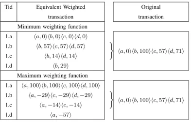
transactional sets associated with each weighted transaction. Consider, for instance, the example dataset reported in Table I. The equivalent versions of the transaction with tid 1 obtained by using the minimum and the maximum weighting functions are reported in the left-hand side of Table IV, where the original transaction and its equivalent versions are put side by side for convenience.
TABLE IV
EQUIVALENT WEIGHTED TRANSACTION ASSOCIATED WITH THE TRANSACTION WITH TID1IN THE EXAMPLE DATASET.
Tid Equivalent Weighted Original transaction transaction Minimum weighting function
1.a ⟨a,0⟩⟨b,0⟩⟨c,0⟩⟨d,0⟩ } ⟨a,0⟩⟨b,100⟩⟨c,57⟩⟨d,71⟩ 1.b ⟨b,57⟩⟨c,57⟩⟨d,57⟩ 1.c ⟨b,14⟩⟨d,14⟩ 1.d ⟨b,29⟩
Maximum weighting function 1.a ⟨a,100⟩⟨b,100⟩⟨c,100⟩⟨d,100⟩ } ⟨a,0⟩⟨b,100⟩⟨c,57⟩⟨d,71⟩ 1.b ⟨a,−29⟩⟨c,−29⟩⟨d,−29⟩ 1.c ⟨a,−14⟩⟨c,−14⟩ 1.d ⟨a,−57⟩
Readers can notice that each transaction in the equivalent datasets only includes equally weighted items. In both cases, the transaction with tid 1 in Table I is mapped to the equivalent transactions with tids 1.a, 1.b, 1.c, and 1.d. When using the minimum weighting function, the equivalence procedure first considers the lowest among the weights occurring in the original transaction as current reference weightwref(e.g., the weight 0 associated with item
ain tid 1) and generates an equivalent transaction of equally weighted items (tid 1.a). Next, an iterative procedure
only considers, for the subsequent steps, the setS of items contained in the original transaction and having weight
strictly higher thanwref (e.g., itemsb,c, anddin tid 1). Items in S are combined in a new equivalent transaction
(tid 1.b). At this stage, the new value of reference weight wref for tid 1.b is equal to the minimum weight among
the items inS reduced by the previous reference weight value (e.g., the minimum between 100 (100-0), 57 (57-0),
is iterated until S is empty. In case the maximum weighting function is adopted, the procedure is analogous, but the highest transaction weight is selected at each step instead of the lowest one. Note that reducing item weights by the local maximum weight may yield negatively weighted equivalent transactions.
The IWI-support of a weighted itemset in a weighted transactional dataset corresponds to the one evaluated on the equivalent dataset. We denote this property as the equivalence property.
Property 3: Equivalence property. Let T be a weighted transactional dataset and T E its equivalent version.
The IWI-support values of an itemsetI inT andT E are equal.
Proof:Lettq∈T be a weighted transaction covered byI andT Eq={te1, . . . , tek}its equivalent transaction
set. Letmatched={⟨ij, wqj⟩ ∈tq| ij∈I} be the set of matched weighted items andIS(tq)andIS(tep)the set
of items intq andtep, respectively. Consider the IWI-support-min measure first. Let ⟨il, wlq⟩ ∈ matched be the
least weighted item inmatched. By Definition 2, the following equality holds:Wmin(I, tq)=w
q
l. Furthermore, by
Definition 4, any transactiontep∈T Eq containing il includes all the other items in matchedas well. Thus, the
IWI-support-min ofIinT Eq could be rewritten as follows:
∑ tep|il∈IS(tep)Wmin(I, tep)=w q l=Wmin(I, tq). Hence, IWI-support-min(I,T E) =∑T Eq∈T EIWI-support-min(I, T Eq)= ∑
tep∈T Eq|I⊆IS(tep)∧T Eq∈T EWmin(I, tep) = ∑tq∈T|I⊆IS(tq)Wmin(I, tq)= IWI-support-min(I, T).
Consider now the IWI-support-max measure. Let⟨ih, whq⟩ ∈ matchedbe the maximally weighted item inmatched.
By Definition 2, the following equality holds: Wmax(I, tq)=wqh. Furthermore, by Definition 4,
∑
tep|ih∈IS(tep)Wmax(I, tep)=w q
h=Wmax(I, tq). Hence, IWI-support-max(I,T E) = IWI-support-max(I,T) follows
analogously to the former case.
Complexity analysis.The dataset transformation procedure generates, for each transaction, a number of equivalent transactions at most equal to the original transaction length. A lower number of equivalent transactions is generated when two or more items have the same weight in the original transaction. The product of the original dataset cardinality and itslongesttransaction length can be considered a preliminary upper bound estimate of the equivalent dataset cardinality. However, in real datasets many transactions are usually shorter than the longest one and many items have equal weight in the same transaction. This reduces the number of generated equivalent transactions significantly. As confirmed by the experimental results achieved on real and synthetic data (see Section V), the scaling factor becomes actually lower than theaveragetransaction length, which could be considered a more realistic upper bound estimate.
IWI Miner and MIWI Miner exploit the equivalence property to address tasks (A) and (B), stated in Section III, efficiently and effectively. In the following section a thorough description of the proposed algorithms is given.
B. The Infrequent Weighted Itemset Miner algorithm
Given a weighted transactional dataset and a maximum IWI-support (IWI-support-min or IWI-support-max)
threshold ξ, the Infrequent Weighted Itemset Miner (IWI Miner) algorithm extracts all IWIs whose IWI-support
Fig. 1. Example of node pruning. Maximum IWI-support thresholdξ=2.5
IWI-support-max thresholds, we will not distinguish between the two IWI-support measure types in the rest of this section.
IWI Miner is a FP-growth-like mining algorithm [10] that performs projection-based itemset mining. Hence, it performs the main FP-growth mining steps: (a) FP-tree creation and (b) recursive itemset mining from the FP-tree index. Unlike FP-Growth, IWI Miner discovers infrequent weighted itemsets instead of frequent (unweighted) ones. To accomplish this task, the following main modifications with respect to FP-growth have been introduced: (i) A novel pruning strategy for pruning part of the search space early and (ii) a slightly modified FP-tree structure, which allows storing the IWI-support value associated with each node.
To cope with weighted data, an equivalent dataset version is generated (Cf. Definition 4) and used to populate the FP-tree structure. The FP-tree is a compact representation of the original dataset residing in main memory [10]. Unlike the traditional FP-tree creation, items in the FP-tree header table are sorted by their IWI-support value instead of by their traditional support value. Furthermore, the insertion of an equivalent weighted transactiontep,
whose items are all characterized by the same weight wtp, requires increasing the weights associated with the
covered tree nodes bywtp rather than1.
To reduce the complexity of the mining process, IWI Miner adopts an FP-tree node pruning strategy to early
discard items (nodes) that could never belong to any itemset satisfying the IWI-support thresholdξ. In particular,
since the IWI-support value of an itemset is at least equal to the one associated with the leaf node of each of its covered paths, then the IWI-support value stored in each leaf node is a lower bound IWI-support estimate for all
itemsets covering the same paths. Hence, an item (i.e., its associated nodes) is pruned if it appears only in tree
paths from the root to a leaf node characterized by IWI-support value greater thanξ. The pruning property could
be formalized as follows.
Property 4: Pruning property.LetT be a weighted transactional dataset and F PT the FP-tree associated with
T. Letibe an arbitrary item andNi={ni1, . . . , nik} the set of nodes associated withiinF PT. If for each path
fromnij∈Ni to a leaf inF PT the leaf node is characterized by an IWI-support value greater thanξthenicannot
be contained in any IWI satisfying the IWI-support constraint.
Algorithm 1 IWI-Miner(T,ξ) Input: T, a weighted transactional dataset
Input: ξ, a maximum IWI-support threshold
Output: F, the set of IWIs satisfyingξ
1: F=∅/* Initialization */
/* ScanT and count the IWI-support of each item */ 2: countItemIWI-support(T)
3: T ree←a new empty FP-tree;/* Create the initial FP-tree fromT */ 4: for allweighted transactiontqinT do
5: T Eq←equivalentTransactionSet(tq)
6: for alltransactiontejinT Eqdo
7: inserttejinT ree
8: end for
9: end for
10: F ←IWIMining(T ree,ξ, null) 11: return F
by an IWI-support greater thanξ. Hence, for every pathpil from the FP-tree root to a leaf throughnij ∈Ni the
leaf node is characterized by an IWI-support higher thanξ. Consider now a generic itemsetIil composed of items
inpil. Since the IWI-support of the leaf node of pil is greater than ξ then the IWI-support of Iil is greater than ξ, i.e.,Iil does not satisfy the maximum IWI-support constraint. Thus, every itemset containingidoes not satisfy ξ.
Consider, for example, the FP-tree in Figure 1(a) and suppose discovering IWIs by enforcing an IWI-support-min thresholdξequal to 2.5. Itemdis included in the paths{d,c}and{h,d,f}, whose leaf nodes have IWI-support equal
to 3 and 4, respectively (see Figure 1(a)). Sincedis contained only in paths whose leaf nodes have an IWI-support
value greater thanξ, it can be pruned. The same consideration holds forf andh. Instead,b is contained in a path
({a,b,c}) associated with a leaf node having an IWI-support value lower thanξ. Thus, it should be kept. In fact,
{a,b,c} is an IWI characterized by an IWI-support-min equal to 2. The result of the pruning step is reported in
Figure 1(b).
1) Algorithm pseudocode: In Algorithm 1 the IWI Miner pseudocode is reported. The first steps (lines 2-9
of Algorithm 1) generate the FP-tree associated with the input weighted dataset T. Then, the recursive mining
process is invoked on the constructed FP-tree (line 10). The FP-tree is initially populated with the set of equivalent
transactions generated from T. For each weighted transaction tq ∈T the equivalent set (line 5) is generated by
applying functionequivalentTransactionSet, which implements the transactional dataset equivalence transformation
described in Section IV-A.
Once a compact FP-tree representation of the weighted datasetT has been created, the recursive itemset mining
process is executed (Algorithm 1, line 10). A pseudocode of the mining procedure is given in Algorithm 2. Since IWI Miner relies on a projection-based approach [10], items belonging to the header table associated with the input FP-tree are iteratively considered (lines 2-14). Initially, each item is combined with the current prefix to generate
Algorithm 2 IWIMining(T ree,ξ,pref ix) Input: T ree, a FP-tree
Input: ξ, a maximum IWI-support threshold
Input: pref ix, the set of items/projection patterns with respect to whichTreehas been generated
Output: F, the set of IWIs extendingpref ix
1: F=∅
2: for allitemiin the header table ofT reedo
3: I=pref ix∪ {i}/* Generate a new itemsetIby joiningpref ixandiwith IWI-support set to the IWI-support of itemi */ /* IfIis infrequent store it */
4: ifIWI-support(I)≤ξthen
5: F ← F ∪ {I}
6: end if
/* BuildI’s conditional pattern base andI’s conditional FP-tree */ 7: condP atterns←generateConditionalPatterns(T ree,I)
8: T reeI = createFP-tree(condP atterns)
/* Select the items that will never be part of any infrequent itemset */ 9: prunableItems←identifyPrunableItems(T reeI,ξ)
/* Remove fromT reeI the nodes associated with prunable items */
10: T reeI ←pruneItems(T reeI,prunableItems)
11: ifT reeI̸=∅then
12: F ← F ∪IWIMining(T reeI,ξ,I)/* Recursive mining */
13: end if
14: end for
15: return F
a new itemsetI (line 3). IfI is infrequent, then it is stored in the output IWI setF (lines 4-6). Then, the FP-tree
projected with respect to I is generated (lines 7-8) and the IWIMining procedure is recursively applied on the
projected tree to mine all infrequent extensions of I (line 12). Unlike traditional FP-Growth-like algorithms [10],
IWI Miner adopts a different pruning strategy (see lines 9-10). According to Property 4, identifyPrunableItems
procedure visits the FP-tree and identifies items that are only included in paths whose leaves have an IWI-support
aboveξ. Since they cannot be part of any IWI, they are pruned (line 10).
C. The Minimal Infrequent Weighted Itemset Miner algorithm
Given a weighted transactional dataset and a maximum IWI-support (IWI-support-min or IWI-support-max)
thresholdξ, the Minimal Infrequent Weighted Itemset Miner (MIWI Miner) algorithm extracts all the MIWIs that
satisfyξ.
The pseudocode of the MIWI Miner algorithm is similar to the one of IWI Miner, reported in Algorithm 1. Hence, due to space constraints, the pseudocode is not reported. However, in the following, the main differences
with respect to IWI Miner are outlined. At line 10 of Algorithm 1, theMIWIMining procedure is invoked instead
of IWIMining. The MIWIMining procedure is similar to IWIMining. However, since MIWI Miner focuses on
soon as an infrequent itemset occurs (i.e., immediately after line 5 of Algorithm 2). In fact, whenever an infrequent itemsetI is discovered, all its extensions are not minimal.
V. EXPERIMENTS
We evaluated IWI Miner and MIWI Miner performance by means of a large set of experiments addressing the following issues: (i) Expert-driven validation from real weighted data (Section V-B), (ii) algorithm performance analysis (Section V-C), and (iii) algorithm scalability analysis (Section V-D). All the experiments were performed on a 3.0 GHz Intel Xeon system with 4 GB RAM, running Ubuntu 10.04 LTS. The IWI Miner and MIWI Miner algorithms were implemented in the C++.
A. Dataset description
The characteristics of the evaluated datasets are summarized in the following.
Real-life datasets.To validate the usefulness of the proposed algorithms we analyzed 10 collections, each one composed of 31 real-life weighted datasets. Each collection was obtained by measuring the CPU usage of a multi-core system when executing a different benchmark, among the ones available at http://www.dacapobench.org/. The benchmarks (e.g., avrova, batik) are exploited to analyze multi-core system performance by running a number of standard programs. Each dataset reports the per-core usage rate of a multi-core machine during the execution of a benchmark. In particular, each weighted transaction corresponds to a distinct reading sampled at a fixed point of time, where its weighted items represent the per-core usage rate measures. Datasets have been populated by performing tests on a IBM Power7 machine equipped with 4 CPUs with 8 cores each and enabling/disabling the available cores. More specifically, for each collection, each of the considered datasets represents the CPU usage collected with a different multi-core setting, i.e., the first dataset is relative to a 2-core setting (i.e., 2 out of 32 cores were enabled, while all the others were temporarily idle), the second one to a 3-core setting, etc. Each dataset is characterized by a number of items per transaction equal to the number of enabled cores, i.e., the transaction length is equal to the number of enabled cores. The sampling rate is around 1 s for the 2-core setting, while it decreases when a larger number of cores is enabled. Hence, the dataset cardinality is usually higher for highly parallelized test settings.
Synthetic datasets. We also exploited a synthetic dataset generator to evaluate algorithm performance and scalability. The data generator is based on the IBM data generator [19]. It allows generating transactional synthetic datasets by setting (i) the dataset cardinality, (ii) the average transaction length, and (iii) the item correlation factor. To assign weights to data generated by the IBM generator we integrated a synthetic weight generator. The newly proposed data generator version may assign to each data item a weight according to two different distributions, chosen as representative among all the possible data distributions, i.e, the uniform data distribution and the Poisson distribution. When not otherwise specified, in the following experiments item weights are selected in the range [1,100]. The synthetic weighted data generator is publicly available at http://dbdmg.polito.it/∼paolo/.
B. Knowledge discovery from real benchmark datasets
Analysis and monitoring of multi-core system usage is commonly devoted to (i) detecting system malfunctioning, (ii) optimizing computational load balancing and resource sharing, and (iii) performing system resizing. To address these issues we focus on analyzing and validating, with the help of a domain expert, the usefulness of the patterns extracted by IWI Miner and MIWI Miner from the real-life datasets described in Section V-A.
Since item weights occurring in the analyzed datasets represent core load rates, IWIs and MIWIs that satisfy a maximum IWI-support value represent combinations of underutilized or idle cores. More specifically, when setting an
IWI-support-min threshold, MIWIs represent the smallest core combinations that containat leastone underutilized
core. Instead, when setting the IWI-support-max threshold, MIWIs represent the smallest core combinations that
containonlyunderutilized cores.
Consider the avrova benchmark first. In Table V the number of MIWIs mined by MIWI Miner by setting different values of the maximum IWI-support-min and IWI-support-max thresholds (relative to 10% and 30% core usage rates, respectively) is reported. Since core usage rates range from 0 to 100, for each dataset the absolute threshold relative to thex% usage rate is given by|T| ·x%, where|T|is the dataset cardinality (i.e., the number of samples). The corresponding values are given in Columns 2 and 5 in Table V. A preliminary analysis of the MIWIs extracted by enforcing different IWI-support-max thresholds shows that, unexpectedly, some cores become underutilized when the workflow is allocated over several cores. For instance, when 7 or more cores are simultaneously enabled some of them have an average usage rate lower than 30% in all sampled points of time, i.e., at least one MIWI is mined. Similarly, when 12 cores are simultaneously active, there exist 3 core combinations composed of cores with average usage rate lower than 10%. Their inspection allows the expert to drive the process of system resizing.
To detect system malfunctioning or analyze the maximum application parallelism, the expert may also perform a worst-case analysis by discovering situations in which the simultaneous enabling of multiple cores may cause one or more cores to remain, possibly in an alternate fashion, completely idle (i.e., usage rate = 0). This situation may be due to either specific scheduling problems (e.g., the scheduler may fail to consider some of the available cores for its internal allocation policy) or running application constraints, which may limit the maximum system parallelism. Table VI reports the number of IWIs and MIWIs mined from the avrova benchmark datasets by setting IWI-support-min to 0. To give a more detailed insight into the characteristics of the extracted MIWIs, in Figure 2 we also reported the per-length distribution of the MIWIs mined from three representative datasets relative to the avrova benchmark (i.e., the 16-, 24-, and 32-core settings) by enforcing an IWI-support-min threshold equal to 0. The extracted IWIs compactly represent the information that, at each sampling time, at least one of the included cores is idle. The extraction of IWIs with length 1 from highly parallel settings (i.e., the 24- and 32-core settings) confirms the hypothesis of suboptimal resource utilization and suggests disabling/reallocation of specific cores. On the other hand, longer IWIs may suggest the presence of an unbalanced load allocation when enabling specific core combinations. Note that longer IWIs are discovered even when lowly parallelized settings (e.g., 16-core) are analyzed. As a drawback, IWIs with IWI-support-min equal to 0 may also contain highly loaded cores. To focus
TABLE V
NUMBER OFMIWIS MINED BYMIWI MINER BY SETTING DIFFERENT VALUES OF MAXIMUMIWI-SUPPORT-MIN ANDIWI-SUPPORT-MAX THRESHOLDξ. AVROVA BENCHMARK.
Usage≤10% Usage≤30%
Dataset Num. MIWIs Num. MIWIs
IWI- IWI- IWI-
IWI-ξ sup-min sup-max ξ sup-min sup-max
D2cores 790 0 0 2340 0 0 D3cores 780 0 0 2250 0 0 D4cores 750 0 0 2310 0 0 D5cores 770 0 0 2340 1 0 D6cores 780 0 0 2370 10 0 D7cores 790 10 0 2400 15 1 D8cores 800 20 0 2460 6 5 D9cores 820 33 0 2850 9 6 D10cores 950 45 0 3000 12 6 D11cores 1000 54 0 2790 10 9 D12cores 930 52 3 2940 11 11 D13cores 980 39 3 3150 12 11 D14cores 1050 59 2 3150 13 12 D15cores 1050 62 3 3180 15 15 D16cores 1060 58 4 3150 15 14 D17cores 1050 50 6 3300 16 15 D18cores 1100 59 6 3300 17 17 D19cores 1100 43 9 3300 18 17 D20cores 1100 61 9 3360 19 19 D21cores 1120 79 8 3360 21 21 D22cores 1120 66 10 3360 22 22 D23cores 1120 84 10 3390 23 23 D24cores 1130 50 14 3450 23 23 D25cores 1150 74 13 3480 25 25 D26cores 1160 73 14 3570 25 25 D27cores 1190 74 15 3480 27 27 D28cores 1160 58 18 3420 28 28 D29cores 1140 51 20 3510 28 27 D30cores 1170 69 19 3480 29 29 D31cores 1160 76 19 3160 30 30 D32cores 1180 84 20 3120 32 32
the attention on the smallest potentially relevant core combinations, the expert chooses to look into the subset of Minimal IWIs. Although the mined IWI set may be hardly manageable for manual inspection, the number of mined MIWIs is, in most cases, orders of magnitude lower (see Table VI).
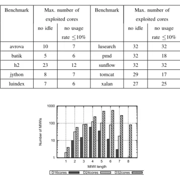
The results confirm that the system has parallelized the computational workflow to lower extent than expected. In fact, idle core situations appear when sampling the system usage with a 14-core setting or higher. Similar results were achieved by evaluating system performance with other benchmarks. Table VII reports, for each tested benchmark, the maximum number of cores yielding an optimal system parallelization in terms of the following
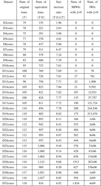
TABLE VI
AVROVA BENCHMARK. NUMBER OFIWIS ANDMIWIS MINED BY SETTING THE MAXIMUMIWI-SUPPORT-MIN THRESHOLDξTO0.
Dataset Num. of Num. of Size Num. of Num. of original equivalent increase MIWIs IWIs
trans. trans. ratio withξ=0 withξ=0
|T| |T E| |T E|/|T| D2cores 79 155 1.96 0 0 D3cores 78 221 2.83 0 0 D4cores 75 291 3.88 0 0 D5cores 77 370 4.81 0 0 D6cores 78 437 5.60 0 0 D7cores 79 511 6.47 0 0 D8cores 80 579 7.24 0 0 D9cores 82 606 7.39 0 0 D10cores 95 723 7.61 0 0 D11cores 100 769 7.69 11 70 D12cores 93 726 7.81 27 781 D13cores 98 756 7.71 42 1,908 D14cores 105 823 7.84 21 9,592 D15cores 105 821 7.82 187 12,931 D16cores 106 824 7.77 135 57,797 D17cores 105 811 7.72 190 121,724 D18cores 110 856 7.78 208 244,546 D19cores 110 882 8.02 175 513,470 D20cores 110 892 8.11 166 1e06 D21cores 112 942 8.41 552 2e06 D22cores 112 947 8.46 484 4e06 D23cores 112 993 8.87 562 8e06 D24cores 113 953 8.43 444 16e06 D25cores 115 1,086 9.44 576 33e06 D26cores 116 1,060 9.14 428 67e06 D27cores 119 1,064 8.94 636 134e06 D28cores 116 1,123 9.68 1513 267e06 D29cores 114 969 8.50 627 536e06 D30cores 117 1,051 8.98 448 1e09 D31cores 116 1,027 8.85 594 2e09 D32cores 118 816 6.92 1,816 4e09
criteria: (A) no idle core is detected, and (B) no core with average usage rate lower than 10% is detected. Condition (A) is verified if no MIWI with IWI-support-min equal to 0 is mined, whereas condition (B) holds when no MIWI with IWI-support-max lower than the 10% usage rate is extracted. The results show that in 7 out of 10 benchmarks there exists at least one core combination for which one or more cores remain idle (not necessarily the same at each instant), and in 8 cases out of 10 there is a suboptimal system resource usage.
TABLE VII
WORKFLOW PARALLELIZATION ANALYSIS.
Benchmark Max. number of Benchmark Max. number of exploited cores exploited cores no idle no usage no idle no usage
rate≤10% rate≤10% avrova 10 7 lusearch 32 32 batik 5 6 pmd 32 18 h2 23 12 sunflow 32 32 jython 8 7 tomcat 29 17 luindex 7 6 xalan 27 25 1 10 100 1000 1 2 3 4 5 6 7 8 Number of MIWIs MIWI length D16cores D24cores D32cores
Fig. 2. Per-length MIWI distribution. Maximum IWI-support-min thresholdξ=0. Avrova benchmark.
C. Performance analysis
We analyzed IWI Miner and MIWI Miner performance on standard synthetic and real datasets. In particular, we analyzed: (i) The impact of the equivalence procedure on the dataset size (see Section V-C1), (ii) the impact of the IWI-support thresholds on both the number of mined patterns and the algorithm execution time (see Section V-C2), and (iii) the comparison, in terms of execution time, between MIWI Miner and MINIT, a state-of-the-art minimal infrequent (unweighted) itemset miner [9] (see Section V-C3).
1) Impact of the equivalence procedure: To enable the IWI mining process from weighted data, an equivalence
procedure, described in Section IV-A, is preliminary applied to the original dataset in order to suit weighted data to the subsequent FP-Growth-like mining step. This section reports the results of an experimental evaluation of the impact of the equivalence procedure on the resulting dataset size.
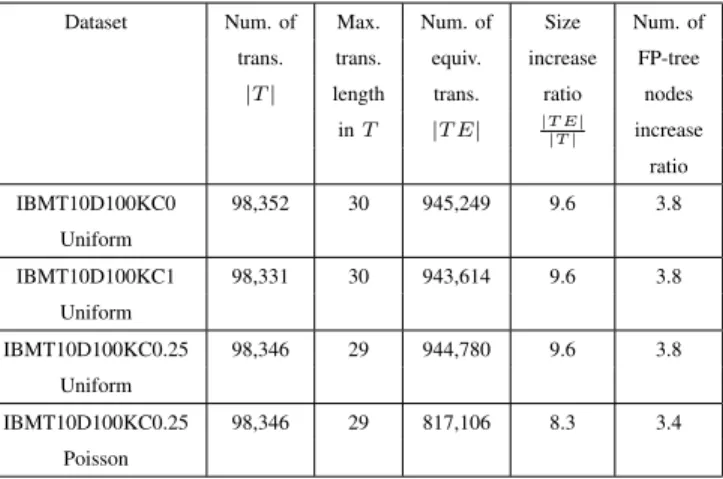
Table VIII reports, for four representative synthetic datasets with different characteristics, the original dataset
size |T| (Column 1), the longest transaction length in T (Column 2), the equivalent dataset size |T E| (Column
3), and the size increase ratio |T E|/|T| (Column 4). In particular, three weighted datasets with size 100,000, average transaction length 10, uniformly distributed weights, and different item correlation values (i.e., minimum (0), standard (0.25), maximum (1)) are considered. Furthermore, one dataset with size 100,000, transaction length 10, Poisson distribution, and standard item correlation value is also analyzed. Similar statistics for the real avrova datasets are given in Table VI.
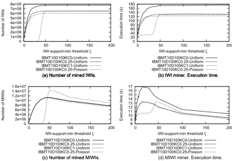
0 1e+09 2e+09 3e+09 4e+09 5e+09 6e+09 7e+09 8e+09 0 50 100 150 200 Number of IWIs IWI-support-min threshold ξ (a) Number of mined IWIs.
IBMT10D100KC0-Uniform IBMT10D100KC0.25-Uniform IBMT10D100KC1-Uniform IBMT10D100KC0.25-Poisson 0 20 40 60 80 100 120 140 160 180 0 50 100 150 200 Execution time (s) IWI-support-min threshold ξ (a) Number of mined IWIs. (b) IWI miner. Execution time.
IBMT10D100KC0-Uniform IBMT10D100KC0.25-Uniform IBMT10D100KC1-Uniform IBMT10D100KC0.25-Poisson 0 2e+06 4e+06 6e+06 8e+06 1e+07 1.2e+07 1.4e+07 1.6e+07 0 50 100 150 200 Number of MIWIs IWI-support-min threshold ξ
(a) Number of mined IWIs. (b) IWI miner. Execution time.
(c) Number of mined MIWIs.
IBMT10D100KC0-Uniform IBMT10D100KC0.25-Uniform IBMT10D100KC1-Uniform IBMT10D100KC0.25-Poisson 8 9 10 11 12 13 14 15 16 17 0 50 100 150 200 Execution time (s) IWI-support-min threshold ξ (a) Number of mined IWIs. (b) IWI miner. Execution time.
(c) Number of mined MIWIs. (d) MIWI miner. Execution time.
IBMT10D100KC0-Uniform IBMT10D100KC0.25-Uniform IBMT10D100KC1-Uniform IBMT10D100KC0.25-Poisson
Fig. 3. Impact of the maximum IWI-support-min threshold on IWI Miner and MIWI Miner performance. IBM synthetic datasets with different data and weight distributions.
0 1e+09 2e+09 3e+09 4e+09 5e+09 6e+09 7e+09 8e+09 0 50 100 150 200 Number of IWIs IWI-support-max threshold ξ
(a) Number of mined IWIs.
IBMT10D100KC0-Uniform IBMT10D100KC0.25-Uniform IBMT10D100KC1-Uniform IBMT10D100KC0.25-Poisson 0 2e+06 4e+06 6e+06 8e+06 1e+07 1.2e+07 1.4e+07 1.6e+07 0 50 100 150 200 Number of MIWIs IWI-support-max threshold ξ
(a) Number of mined IWIs.
(b) Number of mined IWIs.
IBMT10D100KC0-Uniform IBMT10D100KC0.25-Uniform IBMT10D100KC1-Uniform IBMT10D100KC0.25-Poisson
Fig. 4. Impact of the maximum IWI-support-max threshold on IWI Miner and MIWI Miner performance. IBM synthetic datasets with different data and weight distributions.
As discussed in Section IV-A, a more realistic estimate of the number of generated equivalent transactions should consider the average transaction length instead of the maximal one. The results reported in Table VI, achieved on synthetic data with average transaction length 10, confirm the expected trend. However, in practice, since many transactions are shorter than the longest one and many items have the same weight in each transaction, the actual
TABLE VIII
COMPARISON BETWEEN ORIGINAL AND EQUIVALENT DATASETS.
Dataset Num. of Max. Num. of Size Num. of trans. trans. equiv. increase FP-tree
|T| length trans. ratio nodes
inT |T E| |T E||T| increase ratio IBMT10D100KC0 98,352 30 945,249 9.6 3.8 Uniform IBMT10D100KC1 98,331 30 943,614 9.6 3.8 Uniform IBMT10D100KC0.25 98,346 29 944,780 9.6 3.8 Uniform IBMT10D100KC0.25 98,346 29 817,106 8.3 3.4 Poisson
size is significantly lower (e.g., for IBMT10D100KC0.25 the size increase ratio is 9.6 instead of 29). When using the Poisson distribution instead of the uniform one, weights are more correlated with each other and the size increase ratio further decreases (8.3 instead of 29). Similar results come out when coping with real data (e.g., based on the results in Table VI, D32cores achieves 6.92 against 32). As discussed in Section IV-A, a more precise estimate of the number of generated equivalent transactions is obtained by considering the product between the cardinality of T and its average transaction length. In the considered IBM datasets the average transaction length is equal to 10, and its use allows obtaining a good estimate of |T E|.
Since during the FP-Growth-like mining process many transactions may be collapsed into a single FP-tree path, we also analyzed the impact of the equivalent procedure on the FP-tree size. In particular, in Table VI we reported
the ratio between the number of nodes contained in the FP-tree generated from T E and the one relative to the
FP-tree that would be generated fromT (see Column 6). For all the evaluated datasets, the increase ratio, in terms of nodes, is lower than the one achieved in terms of number of transactions because, subsets of equivalent transactions generated from one original transaction are commonly compacted in the same FP-tree path.
2) Impact of the maximum IWI-support threshold: Since IWI-support threshold enforcement may affect the result
of the (M)IWI mining process significantly, we analyzed its impact on IWI Miner and MIWI Miner performance on synthetic data. In particular, we performed different mining sessions, for many combinations of algorithms and datasets with different characteristics, by varying the maximum IWI-support-min and IWI-support-max thresholds. Figures 3(a), 3(c) and 4(a), 4(b) report the number of patterns extracted by IWI Miner and MIWI Miner from datasets with different characteristics by varying the IWI-support-min and IWI-support-max constraints, respectively. For the IWI Miner algorithm, the combinatorial growth of the number of possible infrequent item combinations makes the number of mined IWIs grow super-linearly with the IWI-support threshold until a steady state is reached, because all the possible IWIs have been extracted. Enforcing the support-max constraint instead of the IWI-support-min one yields the curves converging to the steady state condition more slowly, because IWIs have, on
average, higher IWI-support values. Instead, for the MIWI Miner algorithm the combinatorial increase of the number of candidate MIWIs is counteracted by the discarding of some IWIs that become not minimal, i.e., some of their subsets satisfy the IWI-support constraint, from a certain point on. Hence, the total number of MIWIs becomes
maximal at medium IWI-support thresholds (i.e., whenξ is around 25)) while it decreases for higher IWI-support
values.
The average length of the extracted MIWIs also reflects the selectivity of the enforced IWI-support thresholds. In particular, at lower IWI-support thresholds longer MIWIs are selected on average, while the average MIWI length decreases when increasing the maximum IWI-support threshold. As an extreme case, when very high IWI-support thresholds are enforced, only single weighted items get selected as minimal IWIs.
Synthetic datasets with different item correlation factors (i.e., the lowest (0), the highest (1), and the standard one (0.25)) have been generated and tested. Roughly speaking, the correlation factor is an approximation of the dataset density, i.e., the more the items are correlated with each other, the more dense the analyzed data distribution is. As expected, the correlation factor turns out to be inversely correlated with the number of mined (M)IWIs. In fact, denser datasets contain on average a higher number of frequent patterns and, thus, a lower number of infrequent ones.
Weighted datasets with two different weight distributions, i.e., the Poisson distribution with a mean value equal to 50 and the uniform distribution, have also been analyzed. Using the Poisson distribution instead of the Uniform one produces, on average, fewer (M)IWIs with low IWI-support values. In fact, when using Poisson, the distribution of the IWI-supports of the extracted MIWIs is thickened around the mean value 50, while the IWI-supports of the extracted MIWIs are spread across the whole value range when using the uniform distribution.
Since the algorithm execution time and mined set cardinality are strongly correlated each other, the corresponding curves show a similar trend. Hence, due to the lack of space, we report detailed results only for the IWI-support-min measure (Figures 3(b) and 3(d)). Similar results have been obtained by enforcing the IWI-support-max measure.
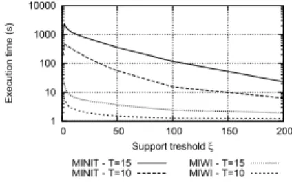
1 10 100 1000 10000 0 50 100 150 200 Execution time (s) Support treshold ξ MINIT - T=15
MINIT - T=10 MIWI - T=15MIWI - T=10
Fig. 5. Comparison between MIWI Miner and MINIT in terms of execution time. Synthetic datasets.
3) Comparison with traditional non-weighted infrequent itemset mining: This paper is, to the best of our
knowledge, the first attempt to perform infrequent itemset mining from weighted data. However, other algorithms (e.g., [7]–[9], [17]) are able to mine infrequent itemsets from unweighted data. Hence, to also analyze the efficiency of the proposed approach when tackling the infrequent itemset mining from unweighted data, we compared
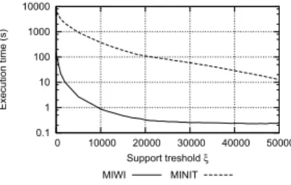
0.1 1 10 100 1000 10000 0 10000 20000 30000 40000 50000 Execution time (s) Support treshold ξ MIWI MINIT
Fig. 6. Comparison between MIWI Miner and MINIT in terms of execution time. Connect UCI dataset.
MIWI Miner execution time with that of a benchmark algorithm, namely MINIT [9]. MINIT is, to the best of our knowledge, the latest algorithm that performs both minimal and non-minimal (unweighted) infrequent itemset mining from unweighted data. For MINIT, we exploited the C++ algorithm implementation available at http://mavdisk.mnsu.edu/haglin. For MIWI Miner, we set all item weights to 1 in order to mine traditional (unweighted) infrequent itemsets.
We compared MIWI Miner and MINIT performance, in terms of execution time, on synthetic and benchmark datasets with different characteristics. Figure 5 reports the execution times achieved by varying the maximum support threshold in the range [0, 200] on two IBM synthetic datasets with 100,000 transactions and two representative average transaction length values (i.e., 10 and 15). The synthetic datasets are characterized by a fairly sparse data distribution. Similarly, Figure 6 reports the results achieved on the real-life Connect dataset downloaded from the UCI repository [20]. Connect is an averagely dense dataset, characterized by 67,557 transactions and 42 categorical attributes, which has already been used for comparing infrequent itemset mining algorithm performance [9]. Since MINIT always takes more than 10 hours in mining non-minimal infrequent itemsets, while IWI Miner execution is orders of magnitude faster, the corresponding plots have been omitted.
Thanks to its FP-growth-like implementation and the applied pruning strategy, MIWI Miner is always at least one order of magnitude faster than MINIT in all the performed comparisons. In particular, when coping with denser datasets (e.g., Connect) MIWI Miner becomes at least two orders of magnitude faster than MINIT for almost all the considered maximum support threshold values. Similar results have been obtained for the other real and synthetic datasets.
For the sake of completeness, we also considered another minimal infrequent mining algorithm, called IFP min [17], beyond MINIT. IFP min is, to the best of our knowledge, the latest minimal (unweighted) infrequent itemset miner. According to the results reported in [17], IFP min is faster than MINIT only when relatively high maximum support
threshold values are enforced. Unlike IFP min, MIWI Miner performs better than MINITfor everysupport threshold
value. Hence, when the mining task becomes more time consuming (i.e., lower support thresholds are enforced) it performs significantly better than both IFP min and MINIT.
In summary, when dealing with unweighted data (i) IWI Miner is shown to be orders of magnitude faster than state-of-the-art algorithms for all considered parameter settings and datasets, and (ii) MIWI Miner is faster or