Gaussian Variational Estimation for Multidimensional Item Response Theory

(1)

Gaussian Variational Estimation

in Multidimensional Item Response Theory

by

April E. Cho

A dissertation submitted in partial fulfillment of the requirements for the degree of

Doctor of Philosophy (Statistics)

in the University of Michigan 2020

Doctoral Committee:

Assistant Professor Gongjun Xu, Chair Assistant Professor Yang Chen

Professor Naisyin Wang

(2)

April E. Cho

[email protected]

ORCID iD: 0000-0003-1818-0399

c

(3)

ACKNOWLEDGEMENTS

First and foremost, I would like to thank my Ph.D. advisor, Professor Gongjun Xu, for his tremendous support and guidance during my graduate study. This work would never have been possible without his help. His guidance is on both academic and personal levels, from which I will benefit for my whole life. Also, I would like to thank my committee members, Professor Naisyin Wang, Professor Yang Chen, and Professor Zhenke Wu, for their advice and insights which helped me greatly improve the quality of my thesis.

My warmest thanks go to my family. I am grateful for their constant love, care and support which made this achievement possible. They are the most important people in my life and I dedicate this thesis to them.

(4)

LIST OF FIGURES

FIGURE

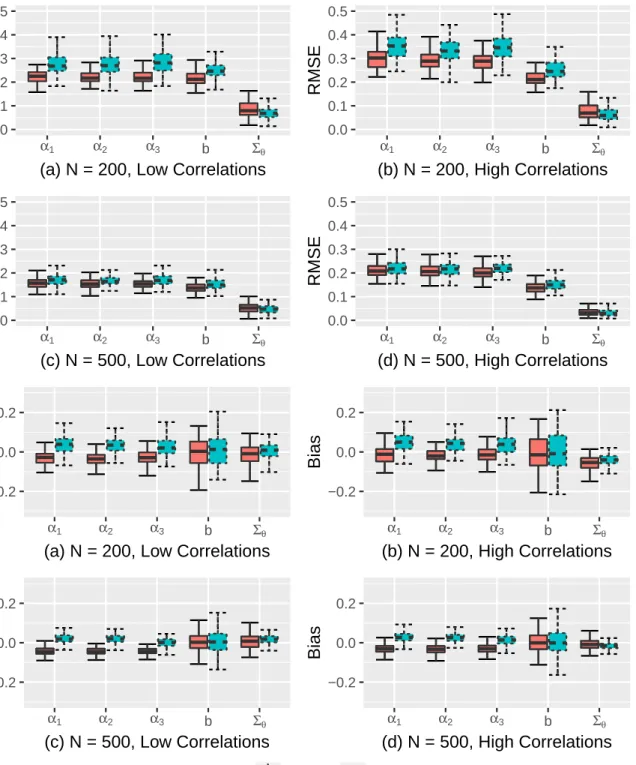
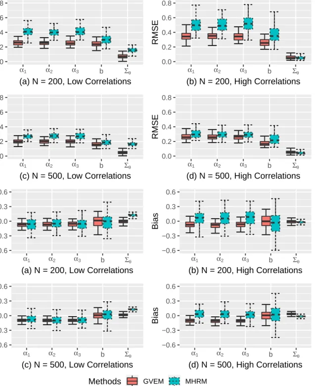
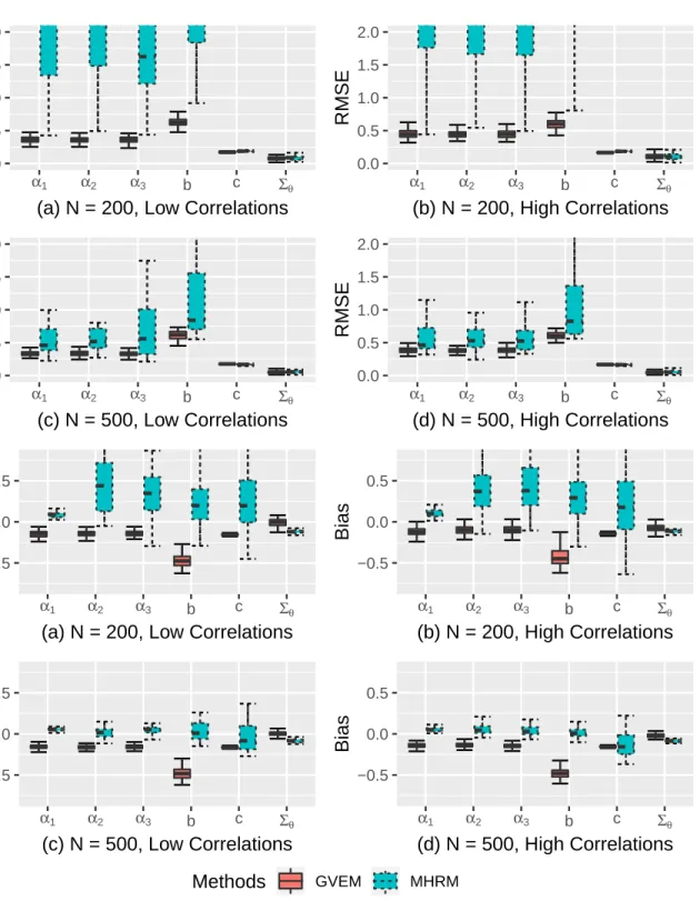
II.1 Parameter recovery of the between-item M2PL models : GVEM vs MHRM . 34

II.2 Parameter recovery of the within-item M2PL models : GVEM vs MHRM . . 35

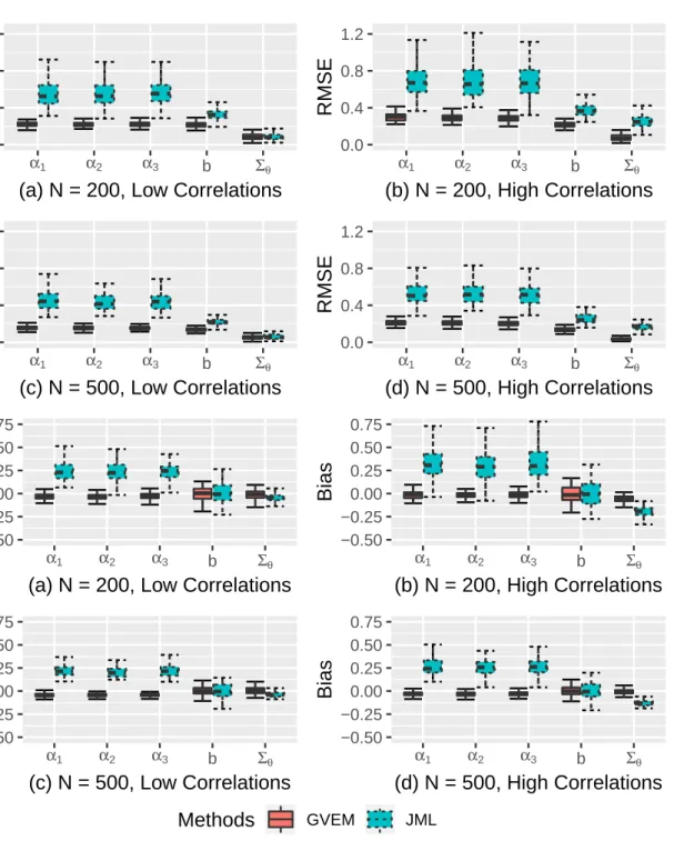
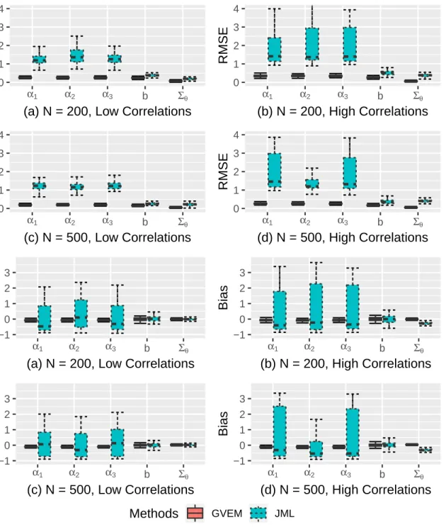
II.3 Parameter recovery of the between-item M2PL models : GVEM vs JML . . 36

II.4 Parameter recovery of the within-item M2PL models : GVEM vs JML . . . 37

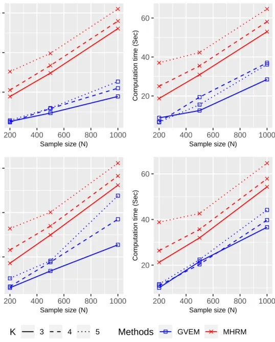
II.5 Average computation time . . . 38

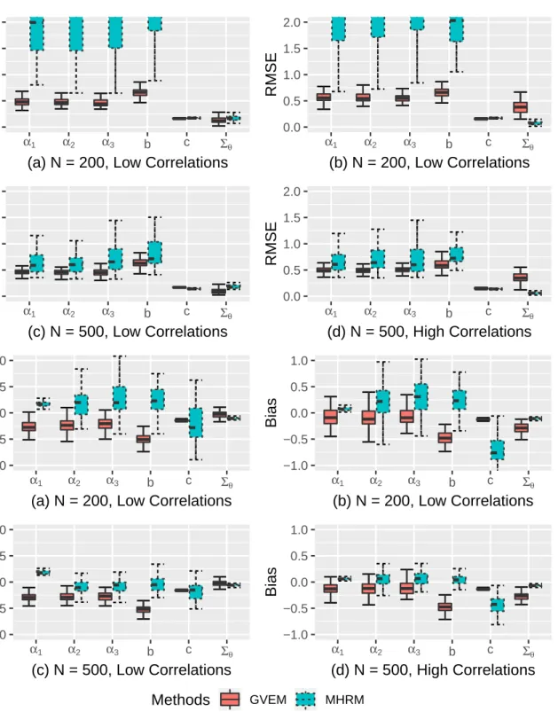
II.6 Parameter recovery of the between-item M3PL models : GVEM vs MHRM . 41

II.7 Parameter recovery of the within-item M3PL models : GVEM vs MHRM . . 42

II.8 Real Data: Model Selection . . . 45

III.1 Correct estimation rates under M2PL. . . 75

III.2 Correct estimation rates under M3PL. . . 75

III.3 Comparison of Lasso and Adaptive Lasso in M2PL under Constraint 1 . . . 76

III.7 Description of questions in science test of NELS:88 . . . 80

(9)

fac-IV.2 Correct Estimation Rates(%) under the between-item multidimensional struc-ture . . . 106

IV.3 Correct Estimation Rates(%) for the within-item multidimensional structure 106

IV.4 False Positive and False Negative rates in between-item model (first row) and within- item model (second row) . . . 107

(10)

LIST OF TABLES

TABLE

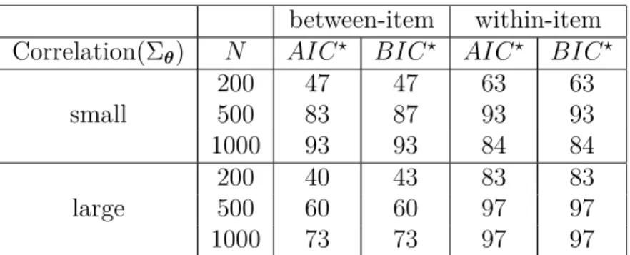
II.1 Correct estimation rate(%) of test dimension in the M2PL model . . . 43

II.2 Correct estimation rate(%) of test dimension in the M3PL model . . . 43

II.3 Real Data: comparison of estimated ˆΣθ . . . 44

III.1 GIC comparison with Adaptive Lasso penalty . . . 79

III.2 Estimated sparse test structure for math test in NELS:88 . . . 82

III.3 Estimated sparse test structure for science test in NELS:88 . . . 83

(11)

LIST OF APPENDICIES

APPENDIX

II.A Derivation of GVEM in the 2PL model . . . 48

II.B Proof of Proposition II.7 . . . 52

II.C Derivation of GVEM in the 3PL model . . . 53

II.D Proof of Theorem II.3 . . . 56

III.A Derivation in M2PL . . . 85

III.B Derivation in M3PL . . . 86

IV.A Derivation of EM steps for M4PL . . . 109

(12)

ABSTRACT

Multidimensional Item Response Theory (MIRT) is widely used in assessment and eval-uation of educational and psychological tests. It models the individual response patterns by specifying functional relationship between individuals’ multiple latent traits and their responses to test items. One major challenge in parameter estimation in MIRT is that the likelihood involves intractable multidimensional integrals due to latent variable structure. Various methods have been proposed that either involve direct numerical approximations to the integrals or Monte Carlo simulations. However, these methods have some limitations in that they are computationally demanding in high dimensions and rely on sampling from a posterior distribution.

In the second chapter of the thesis, we propose a new Gaussian Variational EM (GVEM) algorithm which adopts a variational inference to approximate the intractable marginal like-lihood by a computationally feasible lower bound. The optimal choice of variational lower bound allows us to derive closed-form updates in EM procedure, which makes the algorithm efficient and easily scale to high dimensions. We illustrate that the proposed algorithm can also be applied to assess the dimensionality of the latent traits in an exploratory analysis. Simulation studies and real data analysis are presented to demonstrate the computational efficiency and estimation precision of the GVEM algorithm in comparison to the popular alternative Metropolis-Hastings Robbins-Monro algorithm. In addition, theoretical guar-antees are derived to establish the consistency of the estimator from the proposed GVEM algorithm.

(13)

traits, so-called a test structure. The correct specification of this relationship is crucial for accurate assessment of individuals. Hence, it is of interest to study how to accurately estimate the test structure from data. In the third chapter, we propose to apply GVEM to solve a latent variable selection problem for MIRT and empirically estimate the test structure. The main idea is to impose L1-type penalty to the variational lower bound of the likelihood to recover a simple test structure in iterative procedures. Simulation studies show that the proposed method accurately estimates the test structure and is computationally efficient. A real data analysis on the large-scale assessment test called National Education Longitudinal Study of 1988 is presented.

In the last chapter, we discuss some of the interesting extensions of our proposed method. The first extension is to develop the estimation method via GVEM procedures for the Mul-tidimensional 4-Parameter Logistic model, which is known to be more challenging than previously discussed MIRT models. The second extension is to study Differential Item Func-tioning (DIF) analysis in MIRT. In brief, DIF occurs when groups (such as defined by gender, ethnicity, or education) have different probabilities of responses for a given test item even though people have the same latent abilities. Our goal is to identify test items that have DIF. We formulate the DIF analysis in MIRT as the regularization problem and solve it via our proposed GVEM approach. Simulation studies are presented to show the performance of our proposed method on these topics.

(14)

ChapterI

Introduction

Educational and psychological assessment refers to a way of testing individuals on their latent abilities, characteristics and behavior using combinations of techniques. Its goal is to develop good understanding of the individuals’ latent traits using the observed responses on questionnaires or assessment tests. It is widely used in various fields including education, psychology, and medicine. For example, the proper psychological assessments of individuals would potentially help prepare customized treatments to individuals with mental disorders. In addition, teachers can provide personalized feedback to students and improve the learning process of students. Another interesting application is the online recommender system. The latent preference of online consumers can be measured by analyzing their shopping or viewing history and this could help make predictions for the individualized recommendations. Hence our proposed methods and discussions could be potentially applied in various fields although we mainly focus on the setting of psychological and educational assessment in this dissertation.

The measurement of psychological properties has been a long-lasting quest that origi-nated in the 19th century (Sijtsma & Junker, 2006). Various statistical models have been proposed for psychological assessment since then. Classical test theory (CTT, Gulliksen,

(15)

the 20th century. Fundamental idea of CTT is that the observed test scores contain a true score plus some random error component. That is, CTT assumes that due to random error an observable test score often is not the value representative of a testee’s true performance on the test. The main purpose of CTT is to determine the degree in which test scores are influenced by random error. This has lead to a multitude of methods for estimating the reliability of a test score, of which Cronbach’s alpha (Cronbach, 1951) is the most famous.

CTT was the dominant statistical approach to psychological measurement until the item response theory was introduced (Rasch, 1960; Lord, 1968). Item response theory (IRT) is a general framework for specifying mathematical functions that describe the relationships between individuals’ latent traits and characteristics of test items. Unlike the classical test theory, the item response theory considers the items to be heterogeneous. For example, items may differ in terms of their difficulty levels. IRT is generally regarded as being superior to classical test theory (Embretson & Reise, 2000) and has become the preferred method for developing scales in high-stake tests (e.g. Graduate Record Examination and Graduate Management Admission Test).

The early research on IRT primarily involved unidimensional IRT models that measure only a one latent trait that may represent. As an extension, several multidimensional IRT models have been proposed for modeling the individuals’ response patterns driven by their multiple latent traits (e.g. McKinley & Reckase, 1982; Bock, Gibbons, & Muraki, 1988; Revuelta, 2014). The increasing availability of rich educational and psychological tests has made MIRT an attractive model to handle complex assessment data measuring multiple latent traits at the same time. However, there are some challenges in parameter estimation problem for MIRT. That is, the likelihood involves intractable multidimensional integrals due to multidimensional latent variable structure. With the advancement of computational and statistical techniques, various methods have been proposed that either involve direct numer-ical approximations to the integrals or Monte Carlo simulations. However, these methods still have some limitations in that they are computationally demanding in high dimensions

(16)

and rely on sampling from a posterior distribution. In this thesis, we attempt to tackle the challenging estimation problems in MIRT and develop accurate and efficient estimation algorithms.

The thesis is organized as follows. In the second chapter, we propose a new Gaussian Variational EM (GVEM) algorithm which adopts a variational inference to approximate the intractable marginal likelihood by a computationally feasible lower bound. The optimal choice of variational lower bound allows us to derive closed-form updates in EM procedure, which makes the algorithm efficient and easily scale to high dimensions. We also illustrate that the proposed algorithm can also be applied to assess the dimensionality of the latent traits in an exploratory analysis. A series of simulation studies and real data analysis are presented to demonstrate the performance of the proposed GVEM method in comparison to the popular alternative Metropolis-Hastings Robbins-Monro algorithm. In essence, GVEM method produces more precise parameter estimations and is computational efficient. We also present theoretical guarantees of the estimator from the proposed GVEM algorithm to establish its consistency.

In the third chapter, we propose to apply GVEM to solve a latent variable selection problem for MIRT and empirically estimate the test structure. The test structure illustrates a relationship between the items and the latent traits being measured in a test. The correct specification of this relationship is crucial for accurate assessment of individuals and further model calibration. In practice, practitioners often use fixed test structure based on their prior knowledge for the analysis. However, wrong specification of the relationship would lead to biased estimation. Hence, we would like to study how to accurately estimate the test structure from data. The main idea is to impose L1-type penalty to the variational lower bound of the likelihood to recover a simple test structure in iterative procedures. Simulation studies show that the proposed method accurately estimates the test structure and is computationally efficient. A real data analysis on the large-scale assessment test called

(17)

test design.

In the last chapter, we discuss interesting extensions of our proposed method; (1) to de-velop the estimation method via GVEM procedures for the Multidimensional 4-Parameter Logistic (M4PL) model and (2) to study Differential Item Functioning (DIF) analysis in MIRT. M4PL model has been less preferred so far in the field of education and psychology probably due to its challenge in parameter estimation. In most research, Bayesian approaches with MCMC sampling were used for the parameter estimation in unidimensional 4PL mod-els. However, it gets time consuming for the high dimensional assessment data even for unidimensional latent trait. M4PL models incorporates multiple latent traits at the same time, resulting in intractable multidimensional integrals in the calculation of log-likelihood and making the parameter estimation even more challenging. We develop the variational EM method to facilitate the paraemter estimation in M4PL and discuss the performance with some simulation studies. In the second half of the last chapter, we discuss DIF anlaysis in MIRT. DIF occurs when groups (such as defined by gender, ethnicity, or education) have different probabilities of responses for a given test item even though people have the same latent abilities. Our goal is to identify biasedness in test items (i.e. that have DIF). We formulate the DIF analysis in MIRT as the regularization problem and solve it via our pro-posed GVEM approach. Simulation studies are presented to show the performance of our proposed method on these topics. Lastly we discuss some of the challenges remained and talk about future directions.

(18)

ChapterII

Gaussian Variational EM for

Multidimensional Item Response

Theory

II.1

Introduction

The increasing availability of rich educational survey data and the emerging needs of assess-ing competencies in education pose great challenges to existassess-ing techniques used to handle and analyze the data, in particular when the data are collected from heterogeneous popula-tions. Different forms of multilevel, multidimensional item response theory (MIRT) models have been proposed in the past decades to extract meaningful information from complex education data. The advancement of computational and statistical techniques, such as the adaptive Gaussian quadrature methods, the Metropolis-Hastings Robbins-Monro algorithm, the stochastic expectation maximization algorithm, or the fully Bayesian estimation meth-ods, also help promote the usage of the MIRT models. However, even with these state-of-the-art algorithms, the computation can still be time-consuming, especially when the number

(19)

expectation maximization (GVEM) algorithm for high-dimensional MIRT models.

As summarized in Reckase (2009), the MIRT models contain two or more parameters to describe the interaction between the latent traits and the responses to test items. In this chapter, we focus on the logistic model with dichotomous responses. Specifically for the multidimensional 2-Parameter Logistic (M2PL) model, there are N individuals who respond to J items independently with binary response variables Yij, for i = 1, . . . , N and

j = 1, . . . , J. Then the item response function of theith individual to thejth item is modeled

by

P(Yij = 1|θi) =

exp(α>_j θi−bj) 1 + exp(α>_j θi−bj)

, (II.1)

whereαj denotes aK-dimensional vector of item discrimination parameters for thejth item andbj specifies the corresponding difficulty level with item difficulty parameter asbj/kαjk2.

θi denotes the K-dimensional vector of latent ability for student i.

For the multidimensional 3-Parameter Logistic (M3PL) model, there is an additional parametercj, which denotes the guessing probability of thejth test item. The item response function is expressed as P(Yij = 1|θi) = cj + (1−cj) exp(α>_j θi−bj) 1 + exp(α> jθi−bj) . (II.2)

For both the M2PL and M3PL models, denote all model parameters as Mp. Then given the typical local independence assumption in IRT, the marginal log-likelihood of Mp given the responses Y is l(Mp;Y) = N X i=1 logP(Yi |Mp) = N X i=1 log Z J Y j=1 P(Yij |θi, Mp)φ(θi)dθi. (II.3)

where Yi = (Yij, j = 1, . . . , J) is the ith subject’s response vector and J is the total num-ber of items in the test. The φ denotes the K-dimensional Gaussian distribution of θ with mean 0 and covariance Σθ. The maximum likelihood estimators of the model parameters

(20)

are then obtained from maximizing the log-likelihood function. However, due to the latent variable structure, maximizing the log-likelihood function involves aK dimensional integrals that are usually intractable. Direct numerical approximation to the integrals have been pro-posed in the literature, such as the Gauss–Hermite quadrature (Bock & Aitkin, 1981) and the Laplace approximation (Lindstrom & Bates, 1988; Tierney & Kadane, 1986; Wolfin-ger & O’connell, 1993). However, the Gauss–Hermite quadrature approximation is known to become computationally demanding in the high-dimensional setting, which happens in MIRT especially when the dimension of latent traits increases. The Laplace approximation, though computationally efficient, could become less accurate when the dimension increases or when the likelihood function is in skewed shape. Other numerical approximation meth-ods based on Monte Carlo simulations have also been developed in the literature, such as the Monte Carlo maximization (McCulloch, 1997), stochastic expectation-maximization (von Davier & Sinharay, 2010), Metropolis-Hastings Robbins-Monro algo-rithms (Cai, 2010b, 2010a). These methods usually depends on sampling data points from a posterior distribution and would be computationally involving. Recently, S. Zhang, Chen, and Liu (2020) proposed to use the stochastic EM algorithm (Celeux & Diebolt, 1985) for the item factor analysis, where an adaptive-rejection-based Gibbs sampler is still needed for the stochastic E step. Moreover, Chen, Li, and Zhang (2019) studied the joint maximum likelihood estimation by treating the latent abilities as fixed effect parameters instead of random variables as in (II.3).

In this chapter, we propose a computationally efficient method that is based on the variational approximation to the log-likelihood. Variational approximation methods are mainstream methodology in computer science and statistical learning, and they have been applied to diverse areas including speech recognition, genetic linkage analysis, and document retrieval (Blei & Jordan, 2004; Titterington, 2004). Recently, there is an emerging interest in developing and applying variational methods in statistics (Blei, Kucukelbir, & McAuliffe,

(21)

were developed for standard generalized linear mixed effects models (GLMM) with nested random effects (Ormerod & Wand, 2012; Hall, Ormerod, & Wand, 2011). However, the variational methods have only been slowly recognized in psychometrics and educational measurement, with the pioneer papers by Rijmen and Jeon (2013) as well as Jeon, Rijmen, and Rabe-Hesketh (2017).

In essence, variational approximations refer to a family of deterministic techniques for making approximate inference for parameters in complex statistical models (Ormerod & Wand, 2010). The key is to approximate the intractable integrals (e.g. Eq.(II.3)) with a computational feasible form, known as the variational lower bound to the original marginal likelihood. In psychometrics, Rijmen and Jeon (2013) first developed a variational algorithm for a high dimensional IRT model, but their algorithm was limited to only discrete latent variables. Recently, Jeon et al. (2017) proposed a variational maximization-maximization (VMM) algorithm for maximum likelihood estimation of GLMMs with crossed random ef-fects. They showed that VMM outperformed Laplace approximation with small sample size. However, their study is limited in several respects: (i) They only considered the Rasch model. Although extending their algorithm to the 2PL model may be straightforward, its generalization to 3PL is unknown because 3PL does not belong to the GLMM family; (ii) The key component in their algorithm is the mean-field approximation (Parisi, 1988) that assumes independence of the latent variables given observed data. Even though it seems acceptable to assume independence of each random item effect, this independence assump-tion can no longer apply to the MIRT models when different dimensions are assumed to be correlated; (iii) In their first maximization step, the closed-form solution still contains a two-dimensional integration where adaptive quadrature is used; in the second maximization step, a Newton-Raphson algorithm is used. Therefore, both steps involve iterations, which may slow down the algorithm. Instead, our proposed GVEM algorithm has closed-form solutions for all parameters in both the E and M steps, and it can deal with high-dimensional MIRT models when the multiple latent traits are correlated. Moreover, the GVEM algorithm is

(22)

established for both the M2PL and M3PL models. Consistency theory of the estimators from our proposed algorithm is established, and the performance of the algorithm is thoroughly evaluated via simulation studies.

The rest of the chapter is organized as follows. Section II.2 introduces the general frame-work of the Gaussian Variational method and derivation of EM algorithm in MIRT models. Section II.3 presents the GVEM algorithm for M2PL with the use of local variational ap-proximation and presents the theoretical properties of the proposed algorithm. Section II.4 extends the GVEM algorithm to M3PL and also presents the stochastically optimized algo-rithm to further improve its computational efficiency. Section II.5 and section II.6 illustrate the performance of the proposed GVEM method with simulation studies and on real data, respectively. The chapter is concluded with Section II.7, which discusses any future steps. The Supplementary Material includes the detailed mathematical derivations of the EM steps and the proofs of the theorem and proposition.

II.2

Gaussian Variational EM (GVEM)

From here onwards, for the MIRT models in (II.1) and (II.2), we denote the model parameters

by A={αj, j = 1, . . . , J}, B ={bj, j = 1, . . . , J}, and C ={cj, j = 1, . . . , J}. As defined

in Section II.1, we use the notation Mp ={A,B,C} in the 3PL model and Mp ={A,B} in the 2PL model for simplicity. Latent traits θ from different dimensions are correlated, resulting in a K byK covariance matrix Σθ. To fix the origin and units of measurement, it

is conventional to fix the mean and variance of all θ’s to be 0 or 1, respectively. To remove rotational indeterminacy in the exploratory analysis, (i.e. to ensure the model identifiability) researchers often either assume Σθ = IK or assume A contains a K by K lower triangular matrix (Reckase, 2009).

(23)

In this case, the correlation of latent traits θ is of interest and we need to estimate the covariance matrix Σθ. In this chapter, we consider a general setting of Σθ that works for

both exploratory and confirmatory analyses.

The idea of variational approximation is to approximate the intractable marginal likeli-hood function, which involves integration over the latent random variables, by a computa-tionally feasible lower bound. We follow the approach of variational inference (Bishop, 2006) to derive this lower bound.

The marginal log-likelihood of responses Y is

l(Mp;Y) = N X i=1 logP(Yi |Mp) = N X i=1 log Z J Y j=1 P(Yij |θi, Mp)φ(θi)dθi,

where φ denotes a K-dimensional Gaussian distribution of θ with mean 0 and covariance Σθ. Note that the log-likelihood functionl(Mp;Y) can be equivalently rewritten as

l(Mp;Y) = N X i=1 Z θi logP(Yi |Mp)×qi(θi)dθi,

for any arbitrary probability density function qi satisfying Rθiqi(θi)dθi = 1. Since P(Yi |

Mp) = P(Yi,θi |Mp)/P(θi |Yi, Mp), then we can further write

l(Mp;Y) = N X i=1 Z θi logP(Yi,θi |Mp) P(θi |Yi, Mp) ×qi(θi)dθi = N X i=1 Z θi logP(Yi,θi |Mp)qi(θi) P(θi |Yi, Mp)qi(θi) ×qi(θi)dθi = N X i=1 Z θi logP(Yi,θi |Mp) qi(θi) ×qi(θi)dθi +KL{qi(θi)kP(θi |Yi, Mp)} whereKL{qi(θi)kP(θi |Yi, Mp)}= R θilog qi(θi) P(θi|Yi,Mp)×qi(θi)dθi is the Kullback-Leibler (KL)

distance between the distributionsqi(θi) andP(θi |Yi, Mp). The KL distanceKL{qi(θi)kP(θi |

(24)

have a lower bound of the marginal likelihood as l(Mp;Y) ≥ N X i=1 Z θi logP(Yi,θi |Mp) qi(θi) ×qi(θi)dθi (II.4) = N X i=1 Z θi logP(Yi,θi |Mp)×qi(θi)dθi− N X i=1 Z θi logqi(θi)×qi(θi)dθi

and the equality holds when qi(θi) =P(θi |Yi, Mp) for i= 1, . . . , N.

The follow-up question is how to design the candidate distribution function qi(θi) that gives the best approximation of the marginal likelihood. From the above argument, the best choice is the unknown posterior distribution functionP(θi |Yi, Mp). Although this choice of

qi(θi) is intractable, it provides a guideline to choose qi(θi) in the sense that a good choice of qi(θi) must approximate P(θi | Yi, Mp) well. The well-known EM algorithm follows this idea and can be interpreted as a maximization-maximization (MM) algorithm (Hunter & Lange, 2004) based on the above decomposition. In particular, the E-step chooses qi to be a distribution that minimizes the KL distance function, which corresponds to the estimated posterior distribution P(θi |Yi,Mˆp) with ˆMp from the previous step estimates. The E-step then evaluates the expectation with respect to qi’s, i.e.,

N X i=1 Z θi logP(Yi,θi |Mp)×qi(θi)dθi, (II.5)

which is equal to the lower bound in (II.4), except the additional constant term

−PN

i=1 R

θilogqi(θi)×qi(θi)dθi that does not depend on model parameters Mp. In the

M-step, we maximize the above expectation term to estimate model parameters and this is equivalent to maximizing the lower bound in (II.4).

However, one challenge in the EM algorithm is to evaluate the expectation in (II.5) with respect to the posterior distribution of θi. In the MIRT model, it is known that this integral in (5) does not have an explicit form and in the literature, numerical approximation

(25)

maximization (McCulloch, 1997), and stochastic expectation-maximization (von Davier & Sinharay, 2010).

To avoid directly evaluating the posterior distribution of θi, the variational inference method uses alternative choices of the qi(θi)’s to approximate the marginal likelihood func-tion. The choices of qi(θi) not only approximate the posterior P(θi | Yi, Mp) well, but also are easy to compute and usually give closed form evaluations in the algorithm. In particular, from the MIRT literature, we know that as the number of itemsJ becomes reasonably large, the posterior distribution P(θi | Yi, Mp) can be well approximated by a Gaussian distri-bution (Bishop, 2006). Motivated by this observation, we use the Gaussian approximation procedure that chooses qi(θi) from a family of Gaussian distributions such that the KL dis-tance between qi(θi) and P(θi | Yi, Mp) is minimized. The estimation is then taken as a two-step iterative procedure. In the variational E-step, we choose qi(θi) by minimizing the KL distance betweenqi(θi) and P(θi |Yi, Mp) and evaluate the expectation of the likelihood function with respect qi(θi), which is (II.5). In the M-step we update the unknown model parameters by maximizing the above expectation. The algorithm repeats the two steps until convergence. In the following sections, we present the detailed algorithm steps for the M2PL and M3PL models.

II.3

GVEM for the M2PL Model

In this section we present the GVEM algorithm for the M2PL model. Without loss of generality, we first focus on theith subject’s likelihood function due to the independence of

(26)

different subjects’ responses. The joint distribution function of θi and Yi is logP(Yi,θi |A,B) = logP(Yi |θi,A,B) + logφ(θi) = J X j=1 ( Yijlog exp(α>_jθi−bj) 1 + exp(α>_jθi−bj) + (1−Yij) log 1 1 + exp(α>_j θi−bj) ) + logφ(θi) = J X j=1 ( Yij(α>j θi−bj) + log 1 1 + exp(α>_j θi−bj) ) + logφ(θi).

The difficulty of handling the marginal distribution of Yi mostly comes from the logistic sigmoid function, which makes the integration overθ not in a closed form in the E-step (i.e., Eq. (II.5)).

To avoid dealing with intractable likelihood in E-step, we use a local variational method initially proposed in the machine learning literature (Bishop, 2006; Jordan, Ghahramani, Jaakkola, & Saul, 1999), which finds bounds on functions over individual variables or groups of variables within a model instead of the full posterior distribution over all random variables. For notational simplicity, hereafter, we denotexi,j =bj−α>i θi. Because of the concavity of the logistic sigmoid function log(1/(1 +e−xi,j_{)), by the local variational method we have the}

following result

exi,j

(1 +exi,j₎ = max_ξ_i,j

eξi,j (1 +eξi,j₎exp ( (xi,j−ξi,j) 2 −η(ξi,j)(x 2 i,j−ξ 2 i,j) ) ,

whereξi,j is a variational parameter that is introduced to approximate the objective function

exi,j_/_{(1 +}_exi,j_{), and}

η(ξi,j) = 1 2ξi,j eξi,j (1 +eξi,j₎ − 1 2 .

Therefore, we have the following variational lower bound on the logistic sigmoid function,

exi,j ≥ e ξi,j exp ( (xi,j−ξi,j) −η(ξ )(x2 −ξ2 ) ) . (II.6)

(27)

We then aim to estimate the variational parameter ξi,j that achieves the equality of the above display. By introducing an additional variational parameterξi,j, we successfully avoid the problem of estimating the intractable integral in the E-step. The values of ξi,j’s will be iteratively updated in the M-step.

Using the lower bound on the logistic sigmoid function, we obtain a closed-form lower bound for logP(Yi,θi |A,B) as follows

logP(Yi,θi |A,B) ≥ J X j=1 log e ξi,j (1 +eξi,j₎+ J X j=1 Yij(α>jθi−bj) + J X j=1 (bj−α>j θi−ξi,j) 2 − J X j=1

η(ξi,j){(bj−α>jθi)2−ξi,j2 }+ logφ(θi) =: l(Yi,θi,ξi |A,B)

where ξi = (ξi,j, j = 1, . . . , J)>.

The key step is to find the optimal variational distribution qi(θi), which we describe in detail in the next section.

II.3.1

Algorithm Details

Choice of qi Conditional on the model parameters A,B and the variational parameters

ξi,j for i = 1, . . . , N, j = 1, . . . , J, by the variational inference theory, it can be shown that

the variational distributions qi(θi), i = 1, . . . , N that minimize the KL divergence with the posterior distributionsP(θi|A, B), i= 1, . . . , N take the following form:

logqi(θi) ∝ J X j=1 Yij− 1 2 α>_j θi− J X j=1 η(ξi,j)(bj−α>jθi)2− θ_i>Σ−_θ1θi 2 .

The standard nonlinear optimization technique is exploited to show that qi(θi) ∼ N(θi |

(28)

param-eter is µi = Σi× J X j=1 2η(ξi,j)bj+Yij − 1 2 α>_j (II.7)

and the covariance matrix is determined by

Σ−_i 1 = Σ−_θ1+ 2 J

X

j=1

η(ξi,j)αjα>j . (II.8)

With the variational densities qi(θi)’s, we aim to estimate model parameters ξi’s, αj’s and bj’s by maximizing the lower bound of the marginal likelihood. Suppose we have ξi’s from a previous step’s estimation or the initial values, denoted by ξ_i(t). Similarly, define A(t) ₌_{_α(t) j , j = 1, . . . , J}, B(t) ={b (t) j , j = 1, . . . , J}, Σ (t) θ , µ (t) i and Σ (t) i . The EM iteration is presented below.

E-Step In E-step, we evaluate the closed-form lower bound of the expected log likeli-hood with respect to the variational distributions qi’s. With iteratively updated varia-tional parameters µ(_it) and Σ(_it), we easily evaluate the tth iteration’s lower bound of the expected log-likelihood. Denote the tth iteration’s variational density as q_i(t)(θi) = qi(θi |

ξ_i(t),A(t)_,_B(t)_,_Σ(t)

θ ). Then, thetth iteration’s lower bound can be derived as

E(t)(A,B,ξ) := N X i=1 Z θi l(Yi,θi,ξi |A,B)×q (t) i (θi)dθi = N X i=1 J X j=1 log e ξ_i,j(t) (1 +eξi,j(t)) + (1 2 −Yij)b (t) j + (Yij − 1 2)α (t)> j µ (t) i − 1 2ξ (t) i,j −η(ξ_i,j(t)){b(_jt)2−2b(_jt)α(_jt)>µ(_it)+α_j(t)>[Σ(_it)+ (µ(_it))(µ_i(t))>]α(_jt)−ξ_i,j(t)2} ! +N 2 log|(Σ (t) θ ) −1_{| −} N X i=1 1 2T r((Σ (t) θ ) −1_[Σ(t) i + (µ (t) i )(µ (t) i ) > ]).

(29)

parame-respect to (A,B,ξ,Σθ) to be zero. As a result, it can be shown that each update of the

model parameters are done in a closed form, which makes the proposed GVEM algorithm computationally efficient. The updating step is presented below. The most recently updated copies of the parameters are used for each iterative update.

αj = 1 2

N X

i=1

η(ξi,j)Σi+η(ξi,j)µiµ>i

−1 N X i=1 Yij − 1 2+ 2bjη(ξi,j) µ>_i , (II.9) bj = PN i=1 (1 2 −Yij) + 2η(ξi,j)α > j µi PN i=12η(ξi,j) , (II.10) ξ_i,j2 = b2_j −2bjα>jµi+α>j [Σi +µiµ>i ]αj. (II.11)

For the covariance matrix Σθ, in the exploratory analysis, we can keep Σθ =IK during the GVEM estimation and then later performed proper rotation; in the confirmatory analysis, we update Σθ by Σθ = 1 N N X i=1 [Σi+µiµ>i ]. (II.12)

Note that if the Σθ is assumed to be the correlation matrix with diagonals being 1, then

we need to standardize the estimated Σθ to get correlation matrix. Detailed derivations

regarding the above EM steps are given in the Supplementary Material.

In light of the above exposition, the GVEM algorithm for M2PL can be summarized as follows.

Algorithm 1 GV-EM algorithm 1: Initialize M_p(0) ={A₀,B₀},ξ(0). 2: repeat

3: E step : For step t≥1, updateµ(_it) and Σ(_it) according to closed-form equations (II.7) and (II.8).

4: M step : Further update M_p(t) and ξ(t) according to closed-form equations (II.9), (II.10), and (II.11), iteratively. Fix Σ(_θt) = IK in the exploratory analysis or update Σ(_θt) according to (II.12) in the confirmatory analysis.

(30)

Remark II.1. The algorithm complexity increases with the sample size N, which makes the algorithm computationally inefficient for large data sets. Thus, we can stochastically optimize the EM algorithm by sub-sampling the data to form noisy estimates of the variational lower bound and model parameters. Please refer to Section II.4.2 for detailed explanation of the stochastic GVEM.

Remark II.2. Under the IRT framework, test dimensionality is one of the major issues explored in order to validate the design of a test and help practitioners with test development. As a byproduct of the algorithm, we can empirically estimate the number of latent dimensions from data. Specifically, the information criteria such as AIC or BIC can be used to compare the model fit with varying number of dimensions. Because we approximate the true log-likelihood by its lower bound in GVEM, the information criteria also need to be modified by replacing the true log-likelihood with the variational lower bound, resulting in the following

modified AIC and BIC, denoted as AIC? andBIC?. The approximated information criteria

are as follows, AIC? = 2(kAk0+kBk0+kΣθk0)−2E( ˆA,Bˆ,ξ)ˆ andBIC? =ln(N)(kAk0+

kBk0 +kΣθk0)−2E( ˆA,Bˆ,ξ)ˆ where E( ˆA,Bˆ,ξ)ˆ is the estimated variational lower bound

and Aˆ,Bˆ,ξˆare the final estimates from GVEM estimation procedure. The notation kAk0

of matrix A denotes the zero norm of the matrix A, which is simply the number of

non-zero entries of A. The advantage of using GVEM to estimate test dimensionality is that it

is computationally more efficient especially under high dimensional data and more complex model. This procedure can be easily applied in both the 2PL and the 3PL models. Please see the simulation study for more discussions.

II.3.2

Theoretical Properties

In this section, we establish theoretical bounds on the estimation of the model parameters under the high-dimensional setting where both N and J go to infinity. The dimension of

(31)

denote a matrix of random variables following qi(θi) and let ˆΘ = [ˆθij]N×K denote a matrix of estimated latent abilities from data. Define E_θˆ∼qˆ to be the expectation with respect to

the estimated variational densities {qˆi( ˆθi) ∼N(ˆµi,Σˆi) : i = 1, . . . , N} from data. Lastly, a superscript ∗denote a true parameter. For example, θ_i∗ denotes the ith _{person’s true latent} ability, which is a deterministic realization from its population distribution. We assume that the true parameters Θ∗ and A∗ satisfy

(A1).kθ_i∗k2 _≤_C _and _k_α∗

jk2 ≤C for all i, j for some positive constant C

Theorem II.3 derives the bound on the expected Frobenius norm of the error, kΘ ˆˆA>−

Θ∗(A∗)>kF, where kMkF =

q P

i,jMij2 denotes the Frobenius norm of a matrix M.

Theorem II.3. Suppose that condition (A1) is satisfied for the true parameters Θ∗ and

A∗. With optimally estimated variational densities qˆi from data and estimated parameter

matrix Aˆ that maximizes the variational lower bound, there exists absolute constants C1 and

C2 such that 1 N JEθˆ∼qˆ[k ˆ Θ ˆA>−Θ∗(A∗)>kF]≤C2CeC s J+N J N s 1 + log(N +J) N +J

is satisfied with probability 1−C1/(N +J).

The proof of Theorem II.3 can be found in the Supplementary Material.

Remark II.4. Theorem II.3 states that the expected estimation error measured by Frobenius

norm goes to 0 as both N → ∞ and J → ∞. The proof of Theorem II.3 follows a similar

argument from Davenport, Plan, Van Den Berg, and Wootters (2014) and Theorem 1 in

Chen et al. (2019). However, the previous work by Chen et al. (2019) treats θi as fixed

effects while this work follows the conventional MIRT model setting with θi random effects

and following a normal population distribution.

Remark II.5. The Gaussian family as the candidate choice of q is reasonable according

(32)

of P(θi|Yi) is a normal distribution with MLE θˆi as mean and inverse of observed Fisher

information I−1_{( ˆ}_θ

i)as variance. Denote θi∗ as the true parameter. By Bernstein-von Mises

Theorem, since P(Yi | θi), i = 1, . . . , N have same support and θi → logP(Yi | θi) is

twice continuously differentiable, then θˆi →θi∗ almost surely and the Laplace approximated

distribution N( ˆθi, I−1( ˆθi)) converges in distribution to the true limiting normal distribution

N(θ∗_i, I−1(θ_i∗)) asJ → ∞where I−1(θ∗_i) is the inverse of expected Fisher information. This

supports our choice of variational density qi as a multivariate Gaussian distribution provides

an asymptotically good approximation for the true posterior distribution of θ.

Remark II.6. Compared with the existing stochastic estimation algorithms, such as the Metropolis-Hastings Robbins-Monro algorithm and the stochastic EM algorithm, the proposed estimation method has the advantage that each of the estimation iterations has simple closed-form update and it does not involve the stochastic samplings from some intermediate posterior distributions as in the current stochastic estimation algorithms. As discussed in Remark II.5, even though variational distributions are used to approximate the posterior distributions in our method, the normal approximation is asymptotically valid. Simulation studies in Section II.5 further illustrate this. Moreover, the above variational EM development can be easily generalized to the M3PL model and can also be naturally combined with the idea of the stochastic EM, as illustrated in the next section.

II.4

GVEM for the M3PL Model

Derivation of the variational lower bound is trickier in the M3PL function since the cancella-tion of log and exponential funccancella-tion, which was essential in simplifying the variacancella-tional lower bound in M2PL, is impossible due to the addition of a guessing parameter. To solve this problem, we introduce another latent variable, Zij which is an indicator function of whether

(33)

ability, and Zij = 0 if he or she guessed item j correctly. Notice here that for the case of

Zij = 1, Yij can be either 0 or 1. However, when Zij = 0, Yij has to be 1 by the definition of Zij. Hence, {Yij = 0, Zij = 0} cannot occur.

Proposition II.7. Given the two latent variables θi and Zij, then P(Yij | θi) under the

following hierarchical model is equivalent to (II.2) of the 3PL model.

Zij ∼Bernoulli(1−cj), Yij |θi, Zij = 1 ∼Bernoulli( exp(α> jθi−bj) 1 + exp(α>_jθi−bj) ), Yij |θi, Zij = 0 ∼Bernoulli(I(Yij = 1)).

The distribution of observation Yij given latent variables θi and Zij is then

P(Yij|Zij,θi) = ( exp(α>_j θi−bj) 1 + exp(α> j θi−bj) Yij ₁ 1 + exp(α> j θi−bj) 1−Yij)Zij I(Yij = 1)1−Zij.

Without loss of generality we first focus on the ith subject’s likelihood function due to the independence of different subjects. Denote Zi = {Zi1, Zi2, . . . , ZiJ} and its distribution as

p(Zi) =QJj=1p(Zij). Then the complete data likelihood of the ith subject is

logP(Yi,θi,Zi |A,B,C)

= logP(Yi |θi,Zi,A,B,C) + logφ(θi) + logp(Zi) = J X j=1 ( YijZijlog exp(α> jθi−bj) 1 + exp(α>_j θi−bj) + (1−Yij)Zijlog 1 1 + exp(α>_j θi−bj) ) + J X j=1

{(1−Zij) logI(Yij = 1)}+ logφ(θi) + logp(Zi)

= J X j=1 ( YijZij(α>j θi−bj) +Zijlog 1 1 + exp(α> jθi−bj) + (1−Zij) logI(Yij = 1) )

+ logφ(θi) + logp(Zi).

(34)

with the new latent variable Zij could be used to derive the GVEM algorithm for the 3PL model. Please refer to the Supplementary Material for the proof of Proposition II.7. Similar data augmentation scheme was proposed in Albert (1992) in the Bayesian framework.

In this section, we derive the optimal choices of the variational densities for the latent variables Zij and θi. The approach is similar to that of the 2PL model. For any arbitrary density functions qi and rij of the latent variables θi and Zij, the following equation always holds logP(Yi |A,B,C) = Z θi X Zi

logP(Yi |A,B,C)×qi(θi)ri(Zi)dθi.

where ri(Zi) = QJj=1rij(Zij).

Note that P(Yi | A,B,C) = P(Yi,θi,Zi |A,B,C)/P(θi,Zi |Yi,A,B,C). We can write logP(Yi |A,B,C) = Z θi X Zi log P(Yi,θi,Zi |A,B,C) P(θi,Zi |Yi,A,B,C) ×qi(θi)ri(Zi)dθi = Z θi X Zi log P(Yi,θi,Zi |A,B,C) qi(θi)ri(Zi) ×qi(θi)ri(Zi)dθi +KL{qi(θi)ri(Zi)kP(θi,Zi |Yi,A,B,C)}.

Since the KL distance is ≥0 by definition, we get a lower bound on the marginal likelihood similarly as in the 2PL model.

logP(Yi |A,B,C) ≥

Z

θi

X

Zi

logP(Yi,θi,Zi |A,B,C)×qi(θi)ri(Zi)dθi (II.13)

− Z θi X Zi logqi(θi)ri(Zi) ×qi(θi)ri(Zi)dθi (II.14)

(35)

of the lower bound. Again, theith subject’s likelihood function is logP(Yi,θi,Zi |A,B,C) = J X j=1 ( YijZij(α>j θi−bj) +Zijlog 1 1 + exp(α>_jθi−bj) + (1−Zij) logI(Yij = 1) ) + logφ(θi) + logp(Zi).

Using the same variational lower bound (II.6) on the logistic sigmoid function as in the 2PL model, we show logP(Yi,θi,Zi |A,B,C) ≥ J X j=1 Zijlog eξi,j (1 +eξi,j) + J X j=1 ZijYij(α>j θi−bj) + J X j=1 1 2Zij(bj−α > j θi−ξi,j) − J X j=1 Zijη(ξi,j){(bj −α>j θi)2−ξ2i,j}+ J X j=1 {(1−Zij) logI(Yij = 1)} + logφ(θi) + logp(Zi) =: l(Yi,θi,Zi,ξi |A,B,C).

Recall that if Yij = 0, then we always have Zij = 1 by the design of our model. In other words, {Yij, Zij}={0,0} cannot occur. To accommodate this constraint, we replace Zij by

Z_ij0 = 1−Yij+ZijYij so thatZij0 =Zij ifYij = 1 andZij0 = 1 ifYij = 0. This makes sure that the case of {Yij, Zij} = {0,0} is not included as a possible scenario during the estimation

(36)

procedure. By this substitution, we have l(Yi,θi,Zi,ξi |A,B.C) = J X j=1 (1−Yij+ZijYij) log eξi,j (1 +eξi,j₎ + J X j=1 (1−Yij +ZijYij)Yij(α>j θi−bj) + J X j=1 1 2(1−Yij+ZijYij)(bj −α > j θi−ξi,j) − J X j=1 (1−Yij +ZijYij)η(ξi,j){(bj −α>j θi)2−ξ2i,j} + J X j=1

{Yij(1−Zij) logI(Yij = 1)}+ logφ(θi) + J

X

j=1

logp(Z_ij0 )

where logp(Z_ij0 ) = (1−Yij +ZijYij) log(1−cj) +Yij(1−Zij) log(cj).

With variational distributions qi’s and ri’s, we have the following expression for the variational lower bound of the marginal likelihood, which is an expectation of the joint distribution with respect to qi’s and ri’s, i.e.,

E(t)(A,B,C,ξ) := N X i=1 Z θi " X Zi l(Yi,θi,Zi,ξi |A,B,C)×r (t) i (Zi) # ×q(_it)(θi)dθi. (II.15)

Appropriate choices of the variational distributions will lead to a closed form expression of the lower bound expressed in (II.15). As in the 2PL model, we choose the variational distributions for each latent variable by finding a distribution that best approximates the posterior distribution of each latent variable.

(37)

II.4.1

Algorithm Details

Choice of qi Let Er denote the expectation with respect to. the variational densities of

Zij’s, i.e. rij(Zij)’s. We can write

Er(A,B,C,ξ) := N X i=1 X Zij l(Yi,θi,Zi,ξi |A,B,C)×rij(Zij) = N X i=1 " _J X j=1 (1−Yij +Er[Zij]Yij) log eξi,j (1 +eξi,j) + J X j=1 (1−Yij +Er[Zij]Yij)Yij(α>j θi−bj) + J X j=1 (1−Yij +Er[Zij]Yij) 1 2(bj −α > j θi−ξi,j) − J X j=1 (1−Yij +Er[Zij]Yij)η(ξi,j){(bj −α>j θi)2−ξi,j2 } + J X j=1 {Yij(1−Er[Zij]) logI(Yij = 1)}+ logφ(θi) + J X j=1 Er[logp(Zij0 )] #

Conditional on the model parameters A,B,C and the variational parameters ξi where i=

1, . . . , N, by the variational inference theory, we can show that the variational distributions

qi(θi), i= 1, . . . , N that minimize the distances between them and the posterior distributions

take the following form;

logqi(θi) ∝ J X j=1 (1−Yij +Er(Zij)Yij) Yij − 1 2 α>_jθi − J X j=1 (1−Yij +Er(Zij)Yij))η(ξi,j)(bj−α>j θi) 2₋1 2θ > i Σ −1 θ θi.

The above likelihood function implies thatqi(θi)∼N(θi |µi,Σi) where the mean parameter of the normal distribution is

µi = Σi× J X j=1 2η(ξi,j)bj +Yij − 1 2 (1−Yij +Er(Zij)Yij)α>j (II.16)

(38)

and the covariance matrix is determined by Σ−_i 1 = Σ−_θ1+ 2 J X j=1 (1−Yij +Er(Zij)Yij)η(ξi,j)αjα>j . (II.17)

Choice of rij We follow the similar steps as qi. That is, we take the expectation of the lower bound l(Yi,θi,Zi,ξi | A,B,C) with respect to the variational density of θi, qi(θi) and derive the variational distributions for Zij, i = 1, . . . , N, j = 1, . . . , J. The variational distribution minimizes the distances between them and the posterior distributions of Zij given model parameters A,B,C and the variational parameters ξi.

LetEqdenote the expectation with respect to. the variational densitiesqi’s andEqidenote

the expectation with respect to qi. Taking expectation of the lower bound l(Yi,θi,Zi,ξi | A,B,C) with respect to qi(θi), we have

Eq(A,B,C,ξ) = N X i=1 " _J X j=1 (1−Yij +ZijYij) log eξi,j (1 +eξi,j₎ + J X j=1 (1−Yij +ZijYij)Yij(α>j Eqi[θi]−bj) + J X j=1 (1−Yij +ZijYij) 1 2(bj −α > j Eqi[θi]−ξi,j) − J X j=1 (1−Yij +ZijYij)η(ξi,j){Eqi[(bj −α > j θi)2]−ξi,j2 } + J X j=1 {Yij(1−Zij) logI(Yij = 1)}+Eqi[logφ(θi)] + J X j=1 logp(Z_ij0 ) # (II.18)

This implies that the variational distributions rij(Zij) are

logrij(Zij) ∝ ZijYij " log e ξi,j (1 +eξi,j)+Yij(α > jEqi[θi]−bj) + 1 2(bj −α > jEqi[θi]−ξi,j) −η(ξi,j){Eqi[(bj −α > j θi) 2 ]−ξ_i,j2 }+ log(1−cj) # +Yij(1−Zij) " logI(Yij = 1) + log(cj) #

(39)

Thus, rij(Zij)∼Bernoulli(sij) wheresij = 1 if Yij = 0 and s−_ij1 = 1 + cj 1−cj 1 +eξi,j eξi,j exp −Yij(α>jEqi[θi]−bj) + 1 2(bj −α > j Eqi[θi]−ξi,j)−η(ξi,j){Eqi[(bj −α > j θi)2]−ξi,j2 } (II.19) if Yij = 1 where Eqi[θi] =µi and Eqi[(bj −α > j θi)2] =b2j −2bjα>j µi +α>j[Σi+µiµ>i ]αj. With the chosen qi’s and rij’s, we aim to estimate model parameters ξ, A, B and C, by maximizing the variational lower bound of the marginal likelihood, i.e., (II.15). The EM steps for 3PL model follow the same procedure as in 2PL case.

E-Step In every E step, we choose the optimal variational distributionsqi’s andrij’s, which is equivalent to estimating variational parameters µi, Σi, and sij for every i and j. With iteratively updated variational parameters, (i.e. µ(_it), Σ_i(t), ands(_ijt)) and most recent updates of model parameters (i.e. M(t)

p = {A(t),B(t),C(t)}), we derive a closed form expression of variational lower bound at tth step as follows;

E(t)(A,B,C,ξ) = N X i=1 J X j=1 (1−Yij +s (t) ij Yij) log eξ(i,jt) (1 +eξi,j(t)) + (1 2−Yij)b (t) j + (Yij− 1 2)α (t)> j µ (t) i −1 2ξ (t) i,j −η(ξ (t) i,j){b (t)2 j −2b (t) j α (t)> j µ (t) i + (α (t) j ) > [Σ_i(t)+ (µ(_it))(µ_i(t))>]α(_jt)−ξ_i,j(t)2} ! + N X i=1 J X j=1 Yij(1−s (t) ij ) logI(Yij = 1)− N X i=1 1 2T r((Σ (t) θ ) −1_[Σ(t) i + (µ (t) i )(µ (t) i ) > ]) +N 2 log|(Σ (t) θ ) −1_|₊ N X i=1 J X j=1 {(1−Yij +s (t) ij Yij) log(1−c (t) j ) +Yij(1−s (t) ij ) log(c (t) j )}.

M-Step In this step, we again maximize the E(t)_(A_,_B_,_C_,_{ξ) to update the parameters}

(A,B,C,ξ). This is achieved by setting the derivative of E(t)_(A_,_B_,_C_,_{ξ) with respect to}

(A,B,C,ξ) to be zero. Since we have a closed-form expression of the lower bound, updates of the model parameters are also in closed-form. Detailed derivation is provided in the

(40)

Supplementary Material.

For ξ and Σθ, the update is the same as in 2PL model. For other parameters, we derive

the updating rule by taking derivative of the variational lower boundE(A,B,C,ξ) derived in E step. As a result, we have the following updating rule for αj, bj and cj;

αj = 1 2 N X i=1 (1−Yij+sijYij)η(ξi,j)[Σi+µiµ>i ] −1 × N X i=1 (1−Yij +sijYij) Yij − 1 2 + 2bjη(ξi,j) µ>_i , (II.20) bj = PN i=1(1−Yij+sijYij) (1₂ −Yij) + 2η(ξi,j)α (t)> j µi PN i=12(1−Yij +sijYij)η(ξi,j) , (II.21) cj = PN i=1(Yij −sijYij) PN i=1(1−Yij+sijYij) +PNi=1(Yij −sijYij) = 1 N N X i=1 Yij(1−sij). (II.22)

The Algorithm 2 summarizes the EM steps for GVEM algorithm in M3PL.

Algorithm 2 GV-EM algorithm for M3PL 1: Initialize M_p(0) ={A₀,B₀,C₀},ξ(0). 2: repeat

3: E step : For step t ≥ 1, update variational parameters µ(_it+1), Σ(_it+1), and s(_ijt+1) according to closed-form equations (II.16), (II.17), and (II.19).

4: M step : Further update M_p(t+1) according to closed-form equations (II.20), (II.21), and (II.22) iteratively. Update ξ(t+1) _{and Σ}(t+1)

θ same as in M2PL.

5: until convergence

Remark II.8. The theoretical property of the M3PL is more challenging to derive

rigor-ously due to the addition of the guessing parameters cj’s. From Theorem 2 in Davenport

et al. (2014) we can show that the Hellinger distance of error between estimated probability distributions and the true probability distributions is bounded above. For this discussion, we define Hellinger distance for probability distributions and matrices. Hellinger distance

for two scalars p, q ∈ [0,1] is defined as d2

H(p, q) := (

√

p− √q)2 _{+ (}√₁₋_p₋ √₁₋_q₎2_.