Visually Mining Interesting Patterns in Multivariate Datasets

(1)

Worcester Polytechnic Institute

Digital WPI

Doctoral Dissertations (All Dissertations, All Years) Electronic Theses and Dissertations

2013-01-06

Visually Mining Interesting Patterns in Multivariate

Datasets

Zhenyu Guo

Worcester Polytechnic Institute

Follow this and additional works at:https://digitalcommons.wpi.edu/etd-dissertations

Repository Citation

Guo, Z. (2013).Visually Mining Interesting Patterns in Multivariate Datasets. Retrieved from https://digitalcommons.wpi.edu/etd-dissertations/9

(2)

Visually Mining Interesting Patterns in

Multivariate Datasets

Zhenyu Guo

A PhD Dissertation in Computer Science

Worcester Polytechnic Institute, Worcester, MA

December 2012

Committee Members:

Dr. Matthew O. Ward, Professor, Worcester Polytechnic Institute. Advisor.

Dr. Elke A. Rundensteiner, Professor, Worcester Polytechnic Institute. Co-advisor.

Dr. Carolina Ruiz, Associate Professor, Worcester Polytechnic Institute.

(3)

Abstract

Data mining for patterns and knowledge discovery in multivariate datasets are very impor-tant processes and tasks to help analysts understand the dataset, describe the dataset, and predict unknown data values. However, conventional computer-supported data mining approaches often limit the user from getting involved in the mining process and perform-ing interactions durperform-ing the pattern discovery. Besides, without the visual representation of the extracted knowledge, the analysts can have difficulty explaining and understanding the patterns. Therefore, instead of directly applying automatic data mining techniques, it is necessary to develop appropriate techniques and visualization systems that allow users to interactively perform knowledge discovery, visually examine the patterns, adjust the parameters, and discover more interesting patterns based on their requirements.

In the dissertation, I will discuss different proposed visualization systems to assist analysts in mining patterns and discovering knowledge in multivariate datasets, including the design, implementation, and the evaluation. Three types of different patterns are proposed and discussed, including trends, clusters of subgroups, and local patterns. For trend discovery, the parameter space is visualized to allow the user to visually examine the space and find where good linear patterns exist. For cluster discovery, the user is able to interactively set the query range on a target attribute, and retrieve all the sub-regions that satisfy the user’s requirements. The sub-regions that satisfy the same query and are near each other are grouped and aggregated to form clusters. For local pattern discovery, the patterns for the local sub-region with a focal point and its neighbors are computationally extracted and visually represented. To discover interesting local neighbors, the extracted local patterns are integrated and visually shown to the analysts. Evaluations of the three visualization systems using formal user studies are also performed and discussed.

(4)

Acknowledgements

I would never have been able to finish my dissertation without the guidance of my committee members, help from Xmdv group members, and support from my family.

I would like to express my deepest gratitude to my advisor, Matt, for his excellent guidance, patience, immense knowledge, and for the continuous support of my Ph.D. study and research. His advice and suggestions helped me in all the time of doing re-search, publishing papers, and writing of this thesis. I would like to thank my co-advisor, Elke, who guided me how to conduct thoughtful research and write excellent papers. I am strongly impressed by her enthusiasm and dedicated research attitude, which always encouraged me to seek and perform exciting research to finish my thesis. I would like to thank Prof. Ruiz for her guidance on my directed research. She provided me many useful suggestions to get this work published and this thesis completed. I would also like to thank my external committee member Prof. Grinstein. He devoted a lot time for my comprehensive examination and for my talks. Many thanks for his valuable contributions to this thesis.

I would like to thank Xmdv group members, Zaixian Xie, Di Yang, Abhishek Mukherji, Kaiyu Zhao, and Xika Lin, for the projects and papers we worked together, for the systems we developed together, and also for their broad help during the last four years.

I would also like to thank my parents. They were always encouraging me with their best wishes. Finally, I would like to thank my wife. She was always there supporting me and stood by me through the good times and bad.

(5)

List of Figures

2.1 Visual data mining as a human-centerd interactive analytical and

discov-ery process [58]. . . 9

3.1 A dataset with a simple linear trend: y = 3x1 −4x2 is displayed with parallel coordinates. The axes from left to right are y,x1andx2respectively. 17 3.2 A dataset with two linear trends: y = 3x1−4x2 and y = 4x2 −3x1 is displayed with a scatterplot matrix. . . 17

3.3 The Data Space interface overview. . . 20

3.4 The Model Space interface overview. . . 21

3.5 The Model Space Pattern Selection Panel. . . 22

3.6 The Line Graph of Model Tolerance vs. Percent Coverage. . . 24

3.7 The Orthogonal Projection Plane. . . 24

3.8 The Histogram View. . . 24

3.9 The Projection Plane view before refinement. . . 25

3.10 The Projection Plane view after refinement. . . 25

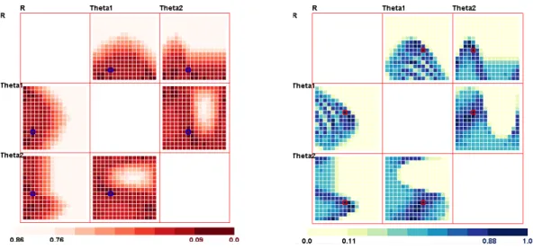
3.11 The Measurement Map: mode is “fix coverage”. . . 27

3.12 The Measurement Map: mode is “fix model tolerance”. . . 27

3.13 The first hot spot is selected representing the first linear trend. . . 28

3.14 The data points that fit the first trend are highlighted in red color. . . 28

3.15 The second hot spot is selected representing another linear trend. . . 28

3.16 The data points that fit the second trend are highlighted in red color. . . . 28

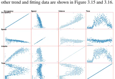
3.17 Traffic dataset data space view (scatterplot matrix). . . 29

3.18 The measurement map with the original color range. . . 30

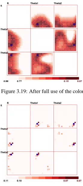
3.19 After full use of the color map. . . 30

3.20 Adjust the color map base point to 0.46. . . 30

3.21 Adjust the color map base point to 0.11. . . 30

3.22 The model space view: a discovered linear trend in a bin center. . . 32

3.23 The corresponding data space view. . . 32

3.24 The model space view: a better linear trend after user adjustment and computational refinement. . . 32

3.25 The corresponding data space view. . . 32

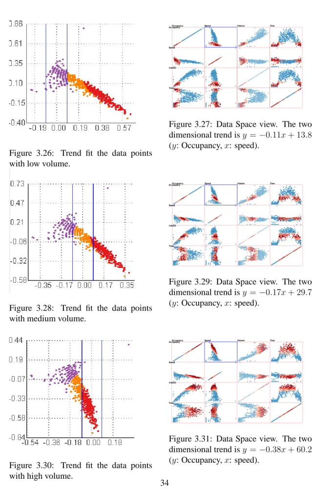
3.26 Trend fit the data points with low volume. . . 34

3.27 Data Space view. The two dimensional trend is y = ₋0.11x+ 13.8 (y: Occupancy,x: speed). . . 34

(8)

3.28 Trend fit the data points with medium volume. . . 34 3.29 Data Space view. The two dimensional trend is y = ₋0.17x+ 29.7(y:

Occupancy,x: speed). . . 34 3.30 Trend fit the data points with high volume. . . 34 3.31 Data Space view. The two dimensional trend is y = ₋0.38x+ 60.2(y:

Occupancy,x: speed). . . 34 3.32 The Orthogonal Projection Plane view after adjusting so that data points

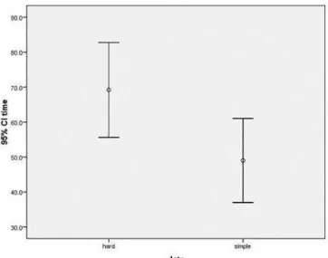
with similar volume align to the linear trend center. Color coding: purple points are low volume; yellow points are median volume; red points are high volume. . . 35 3.33 The comparison of the time the subjects spent on the two dataset: simple

means dataset A and hard means dataset B. . . 37 3.34 The scatterplot for time and error. Each point is one subject. A negative

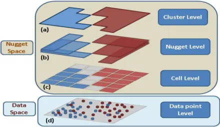
correlation can be seen for these two responses. . . 38 4.1 The 4-level layered Model. User can explore the data space in different

levels in the nugget space. . . 44 4.2 Brushed benign instances . . . 49 4.3 Brushed malignant instances . . . 49 4.4 The mining results are represented in a table before aggregating neighbor

subgroups. . . 50 4.5 The mining results are represented in a table after aggregating neighbour

subgroups. . . 51 4.6 The data space view shows all the nuggets as the translucent bands. The

rightmost dimension is the target attribute. The blue vertical region on the target dimension indicates the target range of the subgroup mining query. 51 4.7 The nugget space view shows the mining result in 3 level of abstractions.

The connecting curves indicate the connection between adjacent levels. . 52 4.8 The comparison of accuracy for different mining result representation types. 54 4.9 The comparison of time for different mining result representation types. . 55 4.10 The comparison of accuracy for different levels. . . 55 4.11 The comparison of time for different levels. . . 56 5.1 The extracted local pattern. . . 62 5.2 The global display using star glyphs (902 records from the diamond dataset).

The color represents whether the data item is an anomalous local pattern or not. The filled star glyphs are selected local pattern neighbors. . . 64 5.3 The local pattern view with a large number of neighbors (332 neighbors),

which results in visual clutter. . . 66 5.4 Neighbor representation using original values. . . 67 5.5 Neighbor representation using comparative values. . . 67

(9)

5.6 The comparison view. The two pink bars in the bottom represent the confidence interval of global pattern (upper) and selected local pattern

(lower). . . 68

5.7 The local pattern adjusting view. The poly-line represents the adjustable coefficients. . . 69

5.8 The local pattern view before adjusting the horsepower coefficient. The neighbor (ID 68) is a worse deal. . . 70

5.9 The local pattern view after adjusting the horsepower coefficient. The neighbor (ID 68) became a better deal. . . 70

5.10 The view for integrating derivatives into global space. The jittered points with different colors indicate the coefficient of∂height/∂weight. As age increases, the coefficient increases. For the same age, the coefficient val-ues are different for different genders. . . 71

5.11 The local pattern view of a gray data item. The orientation from the focal point to all its neighbors areπ/2, which is common in the dataset. . . 72

5.12 The local pattern view of a blue data item. The orientations from the focal point to most of its neighbors are larger thanπ/2, which means the neighbors’ target values are higher than estimated. In other words, the focal point is a “good deal”. . . 73

5.13 The local pattern view of a red data item. The orientations from the focal point to most of its neighbors are lower thanπ/2, which means the neigh-bors’ target values are lower than estimated. In other words, the focal point is a “bad deal”. . . 74

5.14 The coefficients of∂price/∂weightare color-mapped and displayed in a scatterplot matrix of original attribute space. . . 75

5.15 The local pattern view before tuning the coefficients. One neighbor (ID 533) has higher color and the other neighbor (ID 561) has higher clarity. . 76

5.16 The local pattern view after increasing the coefficient of color and de-creasing the coefficient of clarity. The neighbor with higher color became a “good” deal. . . 76

5.17 The local pattern view after decreasing the coefficient of color and in-creasing the coefficient of clarity. The neighbor with higher clarity be-came a “good” deal. . . 76

5.18 The profile glyph display. . . 78

5.19 The star glyph display. . . 78

5.20 The comparison of accuracy for different glyph types. . . 80

5.21 The comparison of time for different glyph types. . . 81

5.22 The comparison of accuracy for different layout types. . . 82

5.23 The comparison of time for different layout types. . . 83

5.24 The local pattern view of diamond 584. . . 85

(10)

List of Tables

5.1 Candidate diamonds after a rough exploration in the global star glyph view. 84 5.2 Candidate diamonds after examining each local pattern of the pre-selected

diamonds. . . 85 6.1 A summary of the three proposed visual mining systems. . . 90

(11)

Chapter 1 Introduction

1.1 Motivation

Knowledge discovery in multivariate databases is “the non-trivial process of identifying valid, novel, potentially useful, and ultimately understandable patterns in data” [26]. The patterns are generally sub-regions or subsets of data points that meet user requirements or satisfy user demands. We use the term “nuggets” to represent discoveries and patterns, which could be clusters, trends, outliers, and other types of sub-regions or subsets that are of interest to users.

Data mining is an important step of the knowledge discovery process, which con-sists of particular mining algorithms to extract and detect hidden patterns in the data. Nowadays, many computational data mining techniques have been proposed, and these techniques become more and more automated, however, user intervention and human un-derstanding are still required to discover novel knowledge. This is true, especially when seeking the answers to some complex analysis questions. In those situations, analysts often integrate their expert knowledge, common sense, intuitions into the data mining process [52]. However, in many cases, conventional automated data mining techniques are often treated as “black-box” systems, which only allow very limited or no user inter-ventions. The limitation of pure automated data mining techniques without visualizations has been discussed in [52].

Moreover, in many cases, the discovered patterns and models only make sense and are explainable when it can be visually represented and examined by the analysts. A vi-sualization system that allows analysts to interactively explore the mined patterns, being aware of the relationships between data space and pattern space, is potentially quite pow-erful. Seeking a more accurate and meaningful pattern, it is more desirable if the users are able to interactively refine and adjust the patterns, based on the users’ task and do-main knowledge. However, this goal is difficult to achieve if the mining process and the extracted patterns are not explicit to the analysts. The potential advantages of visual data mining tools compared to classical data mining tools are discussed in [52] and [19].

In recent years, visualization has been widely used in many data mining process. It can be used to help the analysts explore and navigate the complicated data structures,

(12)

re-veal hidden patterns, and convey the results of data mining [19] [66]. The aim of visual data exploration and mining is to involve the human in the data mining process. Through this, human analysts can apply their perceptual abilities during the analysis, thus gaining a more comprehensive understanding of the mining process and mining results. As dis-cussed in [46], with visual data exploration, the data can be presented in some visual un-derstanding manner, which allows the user to better understand the data, form hypotheses, draw and verify conclusions, as well as perform interactions with the data directly. Keim [45] also argued that visualization techniques are substantially useful for exploratory data analysis and could potentially be very helpful for inspecting large databases, especially in the case where little prior knowledge about the data can be applied.

Visualization can help analysts use visual perception to reveal hidden patterns. The major benefit of visual data exploration is that the users can be directly incorporated in the data mining process. Furthermore, visual analytics can provide an representative and interactive environment, which combines the human’s mental cognitive capabilities and computers’ computing abilities. This can improve both the speed and accuracy when identifying hidden data patterns. The goal of visual data mining, as detailed in [10], is to help analysts establish in-depth insight of the data, to discover novel and useful knowledge from the data, and to acquire a better understanding of the data.

Keim [44] elaborated on the methodology of visual data mining. They pointed out that using visual data exploration has benefits for users, as they can often explore data more efficiently and obtain better results. Visual data exploration is particularly useful when mining tasks are hard to be done solely by automatic algorithms. In addition, as described in [46], another advantage of using visual data exploration techniques is that users could be more confident about their discovered patterns. These advantages promote a high demand of combining visual exploration techniques and automatic exploration techniques together. A variety of visual data exploration and visual data mining techniques were discussed in [20].

In this dissertation, I discussed three novel visualization systems that facilitate vi-sually and computationally discovering and extracting patterns in multivariate datasets. The extracted patterns can be visually represented for better understanding. The users should be able to interactively adjust the pattern based on the user’s task. Visualization systems that integrate the mining process are proposed: from pattern extraction to pattern representation; from pattern examination to pattern refinement.

I list several requirements and desirable features for a visual mining system:

• Understandability requirement: conventional computer-supported data mining

approaches tend to extract complex and incomprehensible patterns, such as a poly-nomial regression line, a neural network, or an arbitrarily-shaped sub-region in high dimensional space. These models can be directly used to solve a classification or a prediction task. However, without an explicit representation and human under-standing, the results are hard to explain and analyze, especially when the output conflicts with domain knowledge or common-sense. The advantages and disadvan-tages of the model are hidden from the user, which may mean the user can only

(13)

passively perform the mining process and accept the mining results without too much critique.

• Visual representation: An effective visualization technique can strongly assist the

analysts in discovering hidden patterns and understanding the data mining results. In most cases, the patterns cannot be directly shown and a particular visualization technique should be designed. For example, in XmdvTool, the hierarchical cluster tree and structure based brush [27] provide a good representation of the clustering results. The designed visual representation should clearly reveal the underlying data structures and convey the extracted patterns using visual components, such as color and line width.

• Refineable and adjustable: When the extracted patterns are not explicit and

vi-sually examinable by the users, they can only generate a new model via adjusting the parameters. However, in most cases, a direct adjustment on the model structure is desirable, for example, removing a branch of a tree structure or changing the coefficient of a regression line.

• Connection between pattern and data: The relationship between the pattern

space and data space should be clearly presented to the analysts. For example, given a regression model, the user needs to know how well the data points fit the model and which points are the outliers. When the users interactively examine dif-ferent sub-parts of the model, the data points that fit or correspond to this sub-part should be highlighted.

• Solve complex real-world application problems: For analysts, data mining

tech-niques and data mining results are considered as a toolbox for solving the real-world problems or answering task-related questions. An example would be that given a classification model, e.g., a classification tree for classifying the paper acceptance results, the users try to figure out why a certain paper is classified as rejected and how to change the attribute values to make it classified as accepted. This example shows that a data mining pattern cannot be directly used to answer users’ guiding questions, except when human intuition and knowledge are involved in the data mining process and pattern exploration.

1.2 Research Goals

In this section, I introduce three topics as my dissertation research goals. Each topic is one type of pattern in multivariate datasets that assists users to understand multi-dimensional phenomena, build models for datasets, and predict target attribute values and class types.

(14)

1.2.1 Linear Trend Patterns

The first challenge is to discover and extract linear patterns from a multivariate dataset. Linear trends are one of the most common patterns and linear regression techniques are widely used to mine these patterns. However, the automatic regression procedure and results pose several problems:

• Lack of efficiency: When discovering trends in a large dataset, users are often only

concerned with a subset of the data that matches a given pattern, so only these data should be used for the computation procedure rather than the whole dataset. Furthermore, locating a good estimation of the trend as an initial input for the re-gression analysis could expedite the convergence, especially for high dimensional datasets.

• Lack of accuracy: Computational results are often not as accurate as the user

ex-pects because users are unable to apply their own domain knowledge and perceptual ability during and after discovering models. User-driven modelling and tuning may be required. For example, an extracted linear trend for a dataset with outliers usu-ally tries to cover all the data points, which means it is not an accurate estimation for inliers.

• Parameter setting problem: Most model estimation techniques require users to

specify parameters, such as the minimum percentage of data points the model in-cludes, maximum error tolerance and iteration count. These are often particular to a concrete dataset, application, and task, but users often don’t know conceptually how to set them.

• Multiple model problem: If multiple phenomena coexist in the same dataset, many

analytic techniques will extract poor models. This is because the computer-based methods try to extract a single model to fit the whole dataset, while in this case, dif-ferent models for difdif-ferent subsets of data points should be extracted. For example, if the linear trends for males and females are different and coexist in the dataset, a single linear trend doesn’t explain the dataset very well. This problem can be solved based on the user’s domain knowledge and visual exploration of the dataset. As part of my dissertation, I developed a system focusing on these problems found in automatic regression techniques. Specifically, I designed a visual interface to allow users to navigate in the model space to discover multiple coexisting linear trends, extract subsets of data fitting a trend, and adjust the computational result visually. The user will be able to select and tune arbitrary high-dimensional linear patterns in a direct and intuitive manner. I designed a sampled model space measurement map that helps users quickly locate interesting exploration areas. While navigating in the model space, the related views that provide metrics for the current selected trend, along with the status of data space, are dynamically displayed and changed, which gives users an accurate estimation to evaluate how well the subset of data fits the trend. The details of this system and the assessing of the technology are discussed in Chapter 3.

(15)

1.2.2 Subgroup Patterns

The second difficulty is to discover interesting subgroups in terms of a target attribute and users’ requirements from a multivariate dataset. Subgroup discovery is a method to discover interesting subgroups of individuals from a multivariate dataset. Subgroups can be described by relations between independent variables and a dependent variable. An interestingness measure, such as a statistical significance value, is also specified to indicate whether the subgroups are of certain interest. Subgroup discovery is used for understanding the relations between a target variable and a set of independent variables.

The subgroup discovery process poses several compelling challenges:

• Dynamically submit queries: since analysts may not know in advance what kind of

interesting features the query results have, they may have to repeatedly re-submit queries and explore the results in multiple passes. This makes the mining process tedious and less efficient.

• Mining results examination problem: without visual support, users can only

exam-ine the mining results in text or tables. This makes it very hard to understand the relationships among different subgroups and how they are distributed in the feature space. A visual representation of the pattern space showing the distribution and relationships among patterns is preferable.

• Compact representation for visualization: the mining results are often reported as

a set of unrelated subgroups. This kind of mining result is not compact because for the adjacent subgroups, they should be aggregated and clustered when they are of the same interesting type. One benefit could be that an aggregate representation is more compact, which provides the users a smaller report list for easy examination. Another benefit could be that the compact representation can be more efficiently stored in a file and loaded in computer memory.

• Relationships between patterns and individuals: without a visualization of the

min-ing results, users cannot build connections between the patterns and the individuals when they explore the mining results. This means that they can only explore the mining result in the form of each subgroup, while they cannot understand the dis-tribution or the structure of the underlying data points.

Focusing on these challenges, our main goal is to design a visual interface allowing users to interactively submit subgroup mining queries for discovering interesting patterns. I proposed and designed a novel pattern extraction and visualization system, called the Nugget Browser, that takes advantage of both data mining methods and interactive visual exploration. Specifically, our system can accept mining queries dynamically, extract a set of hyper-box shaped regions called Nuggets for easy understandability and visualization, and allow users to navigate in multiple views for exploring the query results. While navigating in the spaces, users can specify which level of abstraction they prefer to view. Meanwhile, the linkages between the entities in different levels and the corresponding

(16)

data points in the data space are highlighted. Details and evaluation of this novel system are in Chapter 4.

1.2.3 Local Patterns

The third challenge is to discover and extract interesting local patterns via sensitivity analysis. Sensitivity analysis is the study of the variation of the output of a model as the input of the model changes. Analysts can also discover which input parameters are significant for influencing the output variable. Although many visual analytics systems for sensitivity analysis follow this local analysis method, there are few that allow analysts to explore the local pattern in a pointwise manner, i.e., the relationship between a focal point and its neighbors is generally not visually conveyed. This pointwise exploration is helpful when a user wants to understand the relationship between the focal point and its neighbors, such as the distances and directions.

We seek to propose a novel pointwise local pattern visual exploration method that can be used for sensitivity analysis and, as a general exploration method, for studying any local patterns of multidimensional data. The primary contributions of this work include:

• A pointwise exploration environment: The users should be able to explore a

multi-variate dataset from a pointwise perspective view. This exploration can assist users in understanding the vicinity of a focal point and reveals the relationships between the focal point and its neighbors.

• A visualization approach for sensitivity analysis: Sensitivity analysis is one

im-portant local analysis method, thus is well suited for our pointwise exploration. The designed local pattern exploration view indicates the relationships between the focal point and its neighbors, and whether the relationship conforms to the local pattern or not. This helps the user find potentially interesting neighbors around the focal point, and thus acts as a recommendation system.

• Adjustable sensitivity: The system should allows users to interactively adjust the

sensitivity coefficients, which gives users flexibility to customize their local patterns based on their domain knowledge and goals.

Focusing on these requirements, our main goal is to design a visual interface allowing users to perform pointwise visualization and exploration for visual multivariate analysis. Generally, any local pattern extracted using the neighborhood around a focal point can be explored in a pointwise manner using our system. In particular, we focus on model construction and sensitivity analysis, where each local pattern is extracted based on a regression model and the relationships between the focal point and its neighbors. Using this system, analysts are able to explore the sensitivity information at individual data points. The layout strategy of local patterns can reveal which neighbors are of potential interest. During exploration, analysts can interactively change the local pattern, i.e., the derivative coefficients, to perform sensitivity analysis based on different requirements.

(17)

Following the idea of subgroup mining, we employ a statistical method to assign each local pattern an outlier factor, so that users can quickly identify anomalous local patterns that deviate from the global pattern. Users can also compare the local pattern with the global pattern both visually and statistically. We integrated the local pattern into the original attribute space using color mapping and jittering to reveal the distribution of the partial derivatives. I evaluated the effectiveness of our system based on a real-world dataset and performed a formal user study to better evaluate the effectiveness of the whole framework. Details and evaluation are discussed in Chapter in Section 5.

1.3 Organization of this Dissertation

The following chapters of this dissertation are organized as follows: Chapter 2 proposes related work of visual data mining and visual analytics. Chapter 3 presents a parame-ter space visualization system that allows users to discover linear patparame-terns in multivariate datasets. Chapter 3 describes a visual subgroup mining system, called Nugget Browser, to support users in discovering interesting subgroups with statistical significance in mul-tivariate datasets. Chapter 3 discusses a pointwise local pattern exploration system that assists users in understanding the relationship between the selected focal point and its neighbors, as well as in performing sensitivity analysis. Chapter 6 concludes with a sum-mary and the contributions of this dissertation, as well as potential directions for future research.

(18)

Chapter 2 Related Work

In this chapter, I will give an overview of visual data mining and introduce related works.

2.1 Visual Data Mining Problem

Data Mining (DM) is commonly defined as “the extraction of patterns or models from data, usually as part of a more general process of extracting high-level, potentially useful knowledge, from low-level data”, known as Knowledge Discovery in Databases (KDD) [25], [26]. Data visualization and visual data exploration become more and more impor-tant in the KDD process. Analysts use data mining systems to construct their hypotheses about data sets, which rely heavily on data exploration and data understanding. With interactive navigation of multivariate datasets and query resources, Visual data mining tools allow the analysts to quickly examine their hypotheses, especially for answering the “what if” questions.

The term Visual Data Mining was introduced over a decade ago. The understanding of this term varies for different research groups. “Visual data mining is to help a user to get a feeling for the data, to detect interesting knowledge, and to gain a deep visual understanding of the data set” [10]. Niggemann[51] viewed visual data mining as visual presentation of the data, which is similar to how humans process data presentation. In particular, to understand the data information, humans typically construct a mental model which captures only a gist of the data. A data visualization that is similar to the mental model can reveal hidden information in the data. Ankerst [2] mentioned that visualiza-tion works as a visual representavisualiza-tion of the data. and moreover emphasized the relavisualiza-tion between visualization and the data mining and knowledge discovery (KDD) process. He defined visual data mining as “a step in the KDD process that utilizes visualization as a communication channel between the computer and the user to produce novel and inter-pretable patterns.” Ankerst [2] discussed three different approaches to visual data mining. Two of them involve the visualization of intermediate or final mining results, while the third one, rather than directly being used for showing the results of the algorithm, involves interactive manipulation of the visual representation of the data.

(19)

The above definitions consider that visual data mining is strongly related to the human visual understanding and human cognition. They respectively highlight the importance of the three aspects of visual data mining: (a) data mining tasks; (b) visualization for representation; and (c) data mining process. Overall, integrating the visualization into data mining techniques helps convey mining results in a more understandable manner, deepen the end users’ understanding about how mining techniques work, and manipulate the mining results with human knowledge.

2.2 Visual Data Mining Process

A visual data mining process proposed in [58] is illustrated in Fig. 2.1. The analyst interacts with each step of the pipeline, shown as the bi-directional arrows that connect the analyst and different mining steps. These links indicate that the human analyst plays an important role in the mining process and can be involved in each step. Indicated by thicker bi-directional arrows, data mining algorithms can also be applied to the data in some steps: (a) before any visualization has been carried out, and (b) after interacting with the visualization.

Figure 2.1: Visual data mining as a human-centerd interactive analytical and discovery process [58].

As discussed before, the visual data mining process relies heavily on visualization and interactions. The success of the process depends on the broadness of the collection of vi-sualization techniques. In Fig. 2.1 the “Collection of Vivi-sualization Techniques” are

(20)

com-posed of graphical representations, each of which has some user interaction techniques used for operating with the representation . For instance, in [17], two visual representa-tions were successfully applied to fraud detection in telecommunication data. Keim [43] emphasized further the importance of interactivity of the visual representation, as well as its link to information visualization.

2.3 Visual Data Exploration for Mining

Many application domains have shown examples where parallel coordinates and scat-terplots can be used for exploring the multivariate data. For larger datasets, some user interactions are also incorporated in these techniques, such as selecting and filtering. In-selberg [38] discussed that parallel coordinates transforms the search for relations among different attributes into a 2-D pattern recognition problem. It is also argued that effective user interactions can also be provided for supporting this knowledge discovery process.

The application of a statistical graphics package called XGobi has been described in [59]. They found that visual data mining techniques can be combined together with computational neural modeling, which is a very effective way to detect structures in the neuroanatomical data. This visual data mining tool is used to verify the main hypothesis that neuromorphology shapes neurophysiology. They also discussed that with the fea-ture of brush tour strategy and linked brushing in scatterplots and dotplots, XGobi have been proven as a very successful tool to reveal the hidden structure in their morphology data. As a result, correlation of electrophysiological behavior and certain morphometric parameters are identified and verified.

Hoffman et al. [36] described a case study of using data exploration techniques to classify DNA sequences. Several visual multivariate visualization and data exploration techniques, such as RadViz, Parallel Coordinates, and Sammon Plots [57], have been used to validate and attempt to discover new methods for distinguishing coding DNA se-quences from non-coding DNA sese-quences. Cvek et al. [18] applied visual analytic tech-niques for mining yeast functional genomics datasets. They demonstrated the application of both supervised and unsupervised machine learning to microarray data. Additionally, they presented new techniques that can be used to facilitate clustering comparisons using visual and analytical approaches. They showed that Parallel Coordinates, Circle Seg-ments [5], and RadViz can help gain insight into the data. [28] and [54] also discussed how visual analytic tools can be applied to Bioinformatics, which indicated that this do-main poses many challenges and more and more researchers resort to visual data mining when tackling these challenges.

Recognition of complex dependencies and correlations between variables is also an important issue in data mining. Berchtold et al. [11] proposed a visualization technique called Independence Diagrams, aiming at reveal dependencies among variables. They first divided each variable into ranges. As a result, for each pair of attributes, the com-bination of these ranges can form a two-dimensional grid. For each cell of this grid, the number of data items in it are stored. The grids are visualized via scaling each attribute

(21)

axis. They mapped the the proportional to the total number of data items within that range to the width; and the density of data items in it is mapped to brightness. The authors stated that, with this visual representation, independence diagrams can provide quanti-tative measures of the interaction between two variables. In addition, it allows formal reasoning about issues such as statistical significance. The limitation for this technique is that for each time, only pairs of attributes can be displayed and analyzed.

Classification is another basic task for pattern recognition in data analysis. Dy and Brodley [23] introduced a technique called Visual-FSSEM (Visual Feature Subset Selec-tion using ExpectaSelec-tion-MaximizaSelec-tion Clustering). This method incorporated visualiza-tion techniques, clustering, and user inter- acvisualiza-tion to guide the feature subset search by end users. They chose to display the data and clusterings as 2-D scatterplots projected to the 2-D space using linear discriminant analysis. Visual-FSSEM allowed the users to select any subset of features as a starting point, search forward or backward, and visual-ize the results of the EM clustering, which enables a deeper understanding of the data. In [39], a geometrically motivated classifier is presented and applied, with both training and testing stages, to 3 real datasets. Their implementation allowed the user to select a subset of the available variables and restrict the rule generation to these variables. They stated that the visual aspects can be used for displaying the result as well as exploring the salient features of the distribution of data brought out by the classifier. They tested their classifier on three classification benchmark datasets, and showed very good results as far as test error rates are concerned.

2.4 Visualization of Mining Models

Visualization can also be used to convey the results of mining tasks, which enhances user understanding and user interpretation.

Association rule mining is an important data mining task, which reveals correlations among data items and attribute values. However, understanding the results is not always simple. This is because the mining results are often quite larger than can be handled by humans. Besides, the extracted rules are not generally self-explanatory. Hofmann et al. [37] proposed a method, called Double Decker plots, to visualize the contingency tables to assist the analysts in understanding the underlying structures of association rules. The authors stated that this gives a deeper understanding on the nature of the correlation between the left-hand side of the rule and the right-hand side. An interactive use of these plots are also discussed, which helps the user to understand the relationship between related association rules, for example, for rule sets with a common right-hand side.

Another similar visual representation of multivariate contingency tables is called Mo-saic Plots [33]. A moMo-saic plot is divided into rectangles. The area of each rectangle is proportional to the the number of data items in a cell, i.e., the proportions of the Y variable in each level of the X variable. The arrangement of the rectangles, and how the cells are splitted are determined by both the construction algorithm, as well as the user requirement. The plots reveal the interaction effects between the two variables.

(22)

A commercial DM tool called Mineset was introduced by Brunk et al [14]. In in-tegrated database access, analytical data mining, and data visualization into one system to support exploratory data analysis and visualization of mining results. It provided 3D visualization capabilities for displaying high-dimensional data with geographical and hi-erarchical information. This tool can help identify potentially interesting models of the data using analytical mining algorithms.

Another important data mining results are classifiers that can be used for classification tasks. Some visualization techniques are proposed to support the user’s understanding on the classifiers and manipulate the results. For example, Becker et al. [9] discussed a system called Evidence Visualizer to display the structure of Simple Bayes Models, a decision tree model classifier. This system allowed users to perform interactions, examine specific tree node values, display probabilities of selected items, and ask what if questions during exploration. The reasons for the choices of different visualization techniques, such as pies and bars, are also discussed in detail. Kohavi et al. [47] described a visualization mechanism that are implemented in MineSet to display the decision table classifier. Some interactions were provided for exploration of the classifier, such as clicking to show the next pair of attributes, providing drill-downs to the area of interest.

Han and Cercone [32] emphasized human-machine interaction and visualization dur-ing the entire KDD process. They pointed out that with the human participation in the discovery process, the user can easily provide the system with heuristics and domain knowledge, as well as specify parameters required by the algorithms. They described an interactive system, called CViz, aiming at visualizing the process of classification rule induction. The CViz system uses parallel coordinates technique to visualize the original data and the discretized data. The discovered rules are also visualized as rule polygons (strips) on the parallel coordinates system. The rule accuracy and rule quality were coded by coloring to render the rule polygons. User interaction was supported to allow focusing on subsets of interesting rules. For example, CViz allows user to specify a class label to view all rules that have this class label as the decision value. The users can also use three sliders to hide uninteresting rules: two to set the rule accuracy threshold and one to set quality threshold.

The Self-Organizing Map (SOM) [61] is a neural network algorithm that is based on unsupervised learning. The goal of SOM is to transform an arbitrary dimensional pattern into a one or two dimensional discrete map, which reveals some underlying structure of the data. SOM involves some adaptive learning process, by which the outputs become self-organised in a topologically ordered fashion. In [62], it is discussed that SOM is a widely used algorithm, and it has led to many applications in diverse domains. The authors also argued that SOM can be integrated with different visualization techniques to enhance users’ interpretation.

(23)

2.5 Integrating Visualizations into Analytical Processes

Wong [90] argued: “rather than using visual data exploration and analytical mining algo-rithms as separate tools, a stronger DM strategy would be to tightly couple the visualiza-tions and analytical processes into one DM tool”. Many mining techniques incorporate a variety of mathematical steps, where user intervention is required. However, some min-ing techniques are fairly complex, and visualization plays an important role to support the decision making in the interventions. Standing on this point, the role of a Visual Data Mining technique is considered beyond the traditional belief, that the technique solely participates in some phases of an analytical mining process for exploiting data. Rather, the technique should be viewed as a DM algorithm with visualization as the major role.

A work by Hinneburg et al. is another example that shows the tight coupling of visu-alization into a mining technique [35]. They proposed an approach to effectively cluster high-dimensional data. The approach was established based on combining OptiGrid, an advanced clustering method, and visualization methods to support an interactive cluster-ing procedure. The approach worked in a recursive manner. Specifically, in each step, if certain conditions are met, the actual data set is partitioned into several subsets. Next, for those subsets which contain at least one cluster, the approach deals with them recur-sively, where a new partitioning might take place. The approach chooses a number of separators in regions with minimal point density, and then uses those separators to define a multidimensional grid. For a subset, the recursion stops when no good separators can be found. The difficulty in the approach lies in two aspects: choosing the contracting projec-tions and specifying the separators for constructing the multidimensional grid. These two operations have no way to be done fully automatically due to the diverse cluster charac-teristics in different data sets. The authors resorted to visualization. They developed new techniques that represent the important features of a large number of projections, through which a user can identify the most interesting projections and select the best separators. In this way, the approach improves the effectiveness of the clustering process.

Hellerstein et al. [34] focused on utilizing visualization to improve user control in the process of data discovery. A typical KDD process consists of several steps and require-ments, as well as a sequence of user input for submitting queries and adjusting parameters, which are specific to different algorithms. Some examples are the distance threshold for density based clustering, support and confidence for association rule mining, and the per-centage of training sets for classification. For these continuous user input, visualization can help ease the process. For example, in a time-consuming task, dynamically setting parameters in real time is a highly desirable ability. Statically setting parameters at the beginning of the process could possibly work less efficiently, as whether the settings are reasonable cannot be known until the end of the process.

Ankerst et al. [4], [3] targeted to the problem that the users are unable to be involved in the middle of a running algorithm. The problem is discussed in a classification task that the users cannot get intermediate results. For most current classification algorithms, users have very limited control to guide and interact with the algorithms. They have no other choices aside from running the algorithm with some pre-set, yet typically hard to

(24)

be estimated, parameter values. The users must wait for the final results to tell whether they should have tried some other values. Towards this problem, the authors presented an approach to interactively construct a classifier decision tree. The approach exploits a large amount of visualization for the data set, as well as for the decision tree. Through the enhanced user involvement, the user also gains the benefit of acquiring more insight about the data, during the process of interactive tree construction.

Another similar work is proposed in [65], which emphasized interactive machine learning that involves users in generating the classifier themselves. This allows the users to integrate their background knowledge into the modeling stage and decision tree build-ing process. The authors argued that with the support of a simple two-dimensional vi-sual interface, even common users (not domain experts) can still often construct good classifiers after very little practice. Furthermore, this interactive classifiers construction approach allows users who are familiar with the data to effectively apply their domain knowledge. Some limitations about the approach are also discussed, for example, the manual classifier construction is not likely to be successful for large datasets with large number of attributes to interact with.

Ribarsky et al. [53] propose a mining approach,“discovery visualization”. Unlike the other DM tools, the approach emphasizes user interaction and centers on the users. It uses 4D (time dependent) visual display and interaction to a large degree. In order to smooth the user experience, the approach pays a great amount of attention on organizing data, as it facilitates graphical representation, as well as rapid and accurate selection via the visu-alization. In particular, they present a fast clustering algorithm, that works together with their approach. The algorithm provides users the ability to explore data during continuous adjustment and based on the feedback obtained from the interaction with the visualiza-tion. In addition, the algorithm performs fast clustering with the scalability to very large data sets. It also looks beyond direct spatial clustering and completes the task based on the distribution of other variables. As the first step, the algorithm uses an initial binsort to process the data and maintain them into a more manageable size. Initially, the entire (binsorted) data space is viewed as one big cluster. Next, the data set is divided in a iterative manner, until either a user-specified number of clusters have been formed or it makes no sense to perform further division. This approach enables a quick display for a general overview of the data distribution. The user can select regions of interest and perform further exploration.

My research is strongly related to the visual mining ideas, such as exploration for mining and visually knowledge representation. The main goal of my three visual discov-ery systems is to assist analysts in visually exploring the data space, pattern space, and subgroups to extract and detect certain interesting models or data instances. For example, users are able to explore the parameter space using a linear selection panel to discover strong linear trends, which is discussed in Chapter 3. For each discovered pattern, I de-sign a visual technique, such as a layout strategy of local neighbors discussed in Chapter 5, to help users understand and interpret the extracted knowledge. I also borrow the idea of integrating visualization into mining processes. For example, for the subgroup mining problem mention in Chapter 4, it is difficult to automatically specify the target share range

(25)

and subgroup partitioning strategy because of the diverse dataset characteristics. The sys-tem allows users to dynamically adjust the cut-point positions for binning, and that target share range for different mining tasks they address.

(26)

Chapter 3 Patterns for Linear Trend Discovery

In this chapter, I present a novel visual system that allows analysts to perform the linear model discovery task visually and interactively. This work has been published in VAST 2009 [30].

3.1 Introduction

Discovering and extracting useful insights in a dataset are basic tasks in data analysis. The insights may include clusters, classifications, trends, outliers and so on. Among these, linear trends are one of the most common features of interest. For example, when users attempt to build a model to represent how horsepowerx0and engine sizex1 influence the

retail priceyfor predicting the price for a given car, a simple estimated linear trend model (y =k0x0 +k1x1 +b) could be helpful and revealing. Many computational approaches

for constructing linear models have been developed, such as linear regression [21] and response surface analysis [13]. However, the procedure and results are not always useful for the following reasons:

• Lack of efficiency: When discovering trends in a large dataset, users are often only

concerned with a subset of the data that matches a given pattern, so only these data should be used for the computation procedure rather than the whole dataset. Furthermore, locating a good estimation of the trend as an initial input for the re-gression analysis could expedite the convergence, especially for high dimensional datasets.

• Lack of accuracy: Computational results are often not as accurate as the user

ex-pects because users are unable to apply their own domain knowledge and perceptual ability during and after discovering models. User-driven modeling and tuning may be required.

• Parameter setting problem: Most model estimation techniques require users to

specify parameters, such as the minimum percentage of data points the model in-cludes, maximum error tolerance and iteration count. These are often particular to

(27)

Figure 3.1: A dataset with a simple linear trend: y = 3x1 −4x2 is displayed with

parallel coordinates. The axes from left to right are y,x1 andx2 respectively.

Figure 3.2: A dataset with two linear trends:y= 3x1−4x2andy= 4x2−3x1

is displayed with a scatterplot matrix. a concrete dataset, application, and task, but users often don’t know conceptually how to set them.

• Multiple model problem: If multiple phenomena coexist in the same dataset, many

analytic techniques will extract poor models.

Locating patterns in a multivariate dataset via visualization techniques is very chal-lenging. Parallel coordinates [40] is a widely used approach for revealing high-dimensional geometry and analyzing multivariate datasets. However, parallel coordinates often per-forms poorly when used to discover linear trends. In Figure 3.1, a simple three dimen-sional linear trend is visualized in parallel coordinates. The trend is hardly visible even though no outliers are involved. Scatterplot matrices, on the other hand, can intuitively reveal linear correlations between two variables. However, if the linear trend involves more than two dimensions, it is very difficult to directly recognize the trend. When two or more models coexist in the data (Figure 3.2), scatterplot matrices tend to fail to differ-entiate them.

Given a multivariate dataset, one question is how to visualize the model space for users to discern whether there are clear linear trends or not. If there are, is there a single trend or multiple trends? Are the variables strongly linearly correlated or they just spread loosely in a large space between two linear hyperplane boundaries? How can we visually locate the trend efficiently and measure the trend accurately? How can we adjust arbi-trarily the computational model estimation result based on user knowledge? Can users identify outliers and exclude them to extract the subset of data that fits the trend with a user indicated tolerance? How can we partition the dataset into different subsets fitting different linear trends?

We seek to develop a system focusing on these questions. Specifically, we have de-signed a visual interface allowing users to navigate in the model space to discover multiple

(28)

coexisting linear trends, extract subsets of data fitting a trend, and adjust the computa-tional result visually. The user is able to select and tune arbitrary high-dimensional linear patterns in a direct and intuitive manner. We provide a sampled model space measurement map that helps users quickly locate interesting exploration areas. While navigating in the model space, the related views that provide metrics for the current selected trend, along with the status of data space, are dynamically displayed and changed, which gives users an accurate estimation to evaluate how well the subset of data fits the trend.

The primary contributions of this research include:

• A novel linear model space environment: It supports users in selecting and tuning

any linear trend pattern in model space. Linear patterns of interest can be discovered via interactions that tune the pattern hyperplane position and orientation.

• A novel visualization approach for examining the selected trend: We project

color-coded data points onto a perpendicular hyperplane for users to decide whether this model is a good fit, as well as clearly differentiating outliers. Color conveys the degree to which the data fits the model. A corresponding histogram is also provided, displaying the distribution relative to the trend center.

• A sampled measurement map to visualize the distribution in model space: This

sampled map helps users narrow down their exploration area in the model space. Multiple hot-spots indicate that multiple linear trends coexist in the datasets. Two modes with unambiguous color-coding scheme help users conveniently conduct their navigation tasks. Two color-space interactions are provided to highlight areas of interest.

• Linear trend dataset extraction and management: We present a line graph trend

tolerance selection for users to decide the tolerance (maximum distance error toler-ance from a point to the regression line) for the current model. Users can refine the model using a computational modeling technique after finding a subset of linearly correlated data points. We also allow the user to extract and save data subsets to facilitate further adjustment and examination of their discovery.

3.2 Introduction and System Components

3.2.1 Linear Trend Nugget Definition

We define a nugget as a pattern within a dataset that can be used for reasoning and decision making [67]. A linear trend in n-dimensional space can be represented as(w, X)₋b = 0, whereXi ∈Rndenotes a combination of independent variable vectorxi(xi ∈Rn−1)and

a dependent target valuey(y_∈R). Herewandbare respectively a coefficient vector and a constant value (w _∈ Rn_, _b _∈ _R₎_{. The data points located on this hyperplane construct}

(29)

|(w, x)₋b_|< ε

Considering that noise could exist in all variables (not just the dependent variable), it may be appropriate to use the Euclidean distance from the regression hyperplane in place of the vertical distance error used above [48]. We define a linear trend nugget (LTN) as a subset of the data near the trend center, whose distance from the model hyperplane is less than a certain thresholdE:

LT N(X) =_{x_||(w, x)−b| kw_k < E}

Here E is the maximum distance error, which we call tolerance, for a point to be classified as within the trend. If the distance from a data point to the linear trend hyper-plane is less thanE, it is covered and thus should be included in this nugget. Otherwise it is considered as an outlier or a point that does not fit this trend very well. The two hyperplanes whose offsets from the trend equal E and ₋E construct the boundaries of this trend. The goal of our approach is to help users conveniently discover a “good” linear model, denoted by a small tolerance and, at the same time, covering a high percentage of the data points.

As the range of the values in the coefficient vector could be very large and even in-finite, we transform this linear equation into a normal form to make _kw_k = 1 and then represent this vector asSn_{, a unit vector in hypersphere coordinates [50] as described in}

[22]:

w0 = cos(θ1) w1 = sin(θ1) cos(θ2)

· · ·

wn−2 = sin(θ1)· · ·sin(θn−2) cos(θn−1)

wn−1 = sin(θ1)· · ·sin(θn−2) sin(θn−1)

Now our multivariate linear expression can be expressed as:

ycos(θ1) +x1sin(θ1) cos(θ2) +· · ·+ xn−2sin(θ1) sin(θ2)· · ·sin(θn−2) cos(θn−1)+

xn−1sin(θ1) sin(θ2)· · ·sin(θn−2) sin(θn−1) =r

The last angleθn−1 has a range of 2π and the others have a range of π. The range

of r, the constant value denoting the distance from the origin to the trend hyperplane, is

(0,√n)after normalizing all dimensions.

An arbitrary linear trend can now be represented by a single data point(θ1, θ2,· · ·, θn−1, r)

in the model parameter space. Users can select and adjust any linear pattern in data space by clicking and tuning a point in the model space.

(30)

3.2.2 System Overview

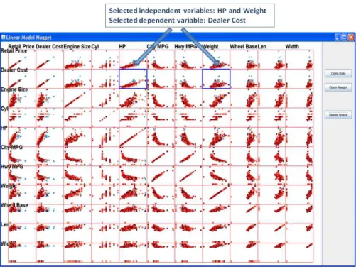
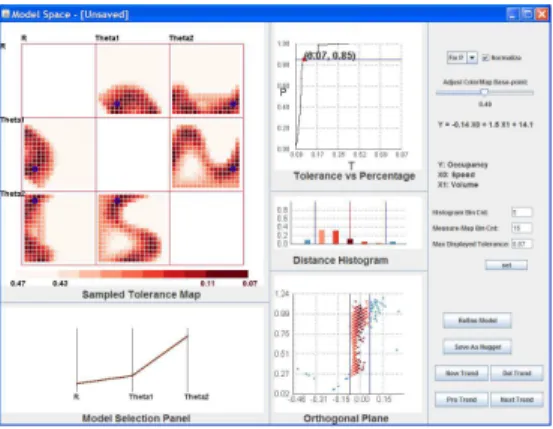
We now briefly introduce the system components and views. The overall interface is depicted in Figures 3.3 and 3.4. The user starts from a data space view displayed with a scatterplot matrix. To explore in the linear model space, the user first indicates the dependent variable and independent variables via clicking several plots in one row. The clicked plots are marked by blue margins; clicking the selected plot again undoes the selection. The selected row is the dependent variable and the columns clicked indicate the independent variables. After the user finishes selecting the dependent and independent variables, he/she clicks the “model space” button to show and navigate in the model space. The points in the data space scatterplot matrix are now colored based on their distance to the currently selected linear trend and dynamically change when the user tunes the trend in the model space. As shown in Figure 3.3, the selected dependent variable is “Dealer Cost” and the two independent variables are “Hp” and “Weight”. The points are color-coded based on the currently selected trend; dark red means near the center and lighter red means further from the center, while blue means the points do not fit the trend. Figure 3.4 is the screen shot of the model space view. Each view in the model space is labeled indicating the components, as described in the following sections.

(31)

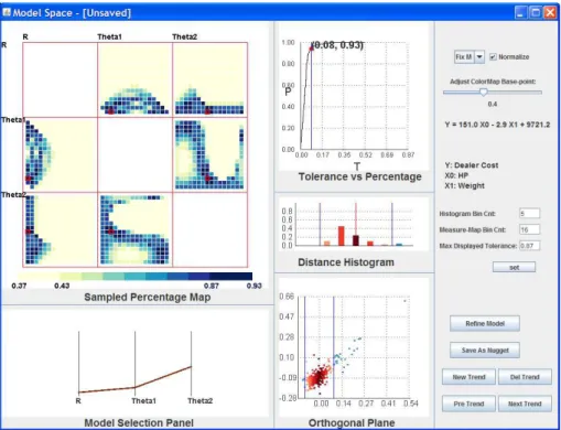
Figure 3.4: The Model Space interface overview.

3.2.3 Linear Trend Selection Panel

We employ Parallel Coordinates (PC), a common visualization method for displaying multivariate datasets [40], for users to select and adjust any linear trend pattern. Each poly-line, representing a single point, describes a linear trend in data space. PC was cho-sen for its ability to display multiple trends at the same time, along with the metrics for each trend. For example, average residual and outlier percentage are easily mapped to poly-line attributes, such as line color and line width. Users can add new trends, delete trends and select trends via buttons in the model space interaction control panel. Users can drag up and down in each dimension axis to adjust parameter values. During dragging, the poly-line attributes (color and width) dynamically change, providing users easy compre-hension of pattern metrics. The parameter value of the current axis is highlighted beside the cursor. This direct selection and exploration allows users to intuitively tune linear pat-terns in model space, sensing the distance from hyperplane to origin as well as the orienta-tions rotated from the axes. Because the parameters in hypersphere coordinates can be dif-ficult to interpret, the familiar formula in the form ofy =k0x0+k1x1+· · ·+kn−1xn−1+b

is calculated and displayed in the interface. In Figure 3.5, three linear trends for a 3-D dataset are displayed. The percentage of data each trend covers (with the same model tolerance) is mapped to the line width and the average residual is mapped to color (dark brown means a large value and light yellow means small).

(32)

Figure 3.5: The Model Space Pattern Selection Panel.

3.2.4 Views for Linear Trend Measurement

When the user tunes a trend in model space, it is necessary to provide detailed information in data space related to the currently selected trend. Based on this the user can differentiate datasets having linear trends from non-linear trends or without any clear trends, as well as discover a good model during tuning. We provide users three related views for discovering trends and deciding the proper model parameters.

Line Graph: Model Tolerance vs. Percent Coverage

For any multi-dimensional linear trend, there is a positive correlation between the tol-erance of the model (the distance between the trend hyperplane and the furthest point considered belonging to the trend) and the percentage of data points this model covers: the larger the model tolerance is, the higher the percentage it covers. There is a trade-off between these two values, because users generally search for models with small tolerance that cover a high percentage of the data. The users expect to find the answer to the follow-ing two questions when decidfollow-ing the model tolerance and percentage it covers: (a) If the model tolerance is decreased, will it lose a large amount of the data? (b) If this trend is expected to cover a greater percentage of the data, will it significantly increase the model tolerance?

To answer these questions, we introduce an interactive line graph for the currently selected model. Model Tolerance vs. Percent Coverage is provided for users to evaluate this model and choose the best model tolerance. It is clear that the line graph curve always goes from (0,0)to (1,1), after normalizing. This line graph also indicates whether this model is a good fit or not. If this curve passes the region near the (0,1) point, there is a strong linear trend existing in the dataset, with a small tolerance and covering a high percentage of the data. This interactive graph also provides a selection function for the model tolerance. The user can drag the point position (marked as a red filled circle in Figure 3.6) along the curve to enlarge or decrease the tolerance to include more or fewer points.

(33)

line graph for a linear trend with about 10 percent outliers is shown. The red point on the curve indicates the current status of model tolerance and percentage. From the curve of the line graph, it is easy to confirm that when dragging the point starting from (0,0)and moving towards(1,1), the model tolerance increases slowly as the percentage increases, meaning that a strong linear trend exists. After moving across 0.90 percent, the model tolerance increases dramatically while the included point percentage hardly increases, indicating that the enlarged model tolerance is mostly picking up outliers. So for this dataset, the user could claim that a strong trend is discovered covering 90 percent of the data points because the model tolerance is very small (0.07). The corresponding Orthogonal Projection Plane view and Histogram view showing the distribution of data points are displayed in Figure 3.7 and Figure 3.8 (described next).

Projection on the Orthogonal Plane

Given an n-dimensional dataset and an n-dimensional linear trend hyperplane, if the user wants to know whether the dataset fits the plane (the distance from points to the hyper-plane is nearly 0), a direct visual approach is to project each data point onto an orthogonal hyperplane and observe whether the result is nearly a straight line.

In particular, we project each high-dimensional data point to a 2-dimensional space and display it in the form of a scatterplot, similar to the Grand Tour [6]. Two projection vectors are required: the first vectorv0is the normal vector of the trend plane, i.e. the unit

vectorwdescribed before; the second vectorv1, which is orthogonal tov0, can be formed

similar to v0, simply by settingθ1 = θ1 +π/2. The positions of data points in the

scat-terplot are generated by the dot products between the data points and the two projection vectors, denoting the distance from the points to the trend hyperplane and another or-thogonal plane, respectively. This view presents the position of each point based on their distance to the current trend, which provides users not only a detailed distribution view based on the current trend, but also the capability of discovering the relative positions of ouliers. Figure 3.7 shows the projection plane. The two blue vertical lines denote the two model boundaries. Data points are color-coded based on their distance to the trend center (not displayed). The red points are data points covered by this trend; darker red means near the center and lighter red means further from the center. The blue points are data that are outliers or ones that do not fit this trend very well.

Linear Distribution Histogram

The histogram view displays the distribution of data points based on their distance to the current model. As shown in Figure 3.8, the middle red line represents the trend center; the right half represents the points above the trend hyperplane, and the left half are those below the trend hyperplane. Users can set the number of bins; the data points included in the trend are partitioned into that number of bins based on their distance to the trend center. The two blue lines represent the boundary hyperplanes. The trend covered bars are red and color-coded according to their distance. The color-mapping scheme is the same

Visually Mining Interesting Patterns in Multivariate Datasets

Worcester Polytechnic Institute

Digital WPI

Visually Mining Interesting Patterns in Multivariate

Datasets

Zhenyu Guo

Visually Mining Interesting Patterns in

Multivariate Datasets

Zhenyu Guo

A PhD Dissertation in Computer Science

Worcester Polytechnic Institute, Worcester, MA

December 2012

Committee Members:

Dr. Matthew O. Ward, Professor, Worcester Polytechnic Institute. Advisor.

Dr. Elke A. Rundensteiner, Professor, Worcester Polytechnic Institute. Co-advisor.

Dr. Carolina Ruiz, Associate Professor, Worcester Polytechnic Institute.

Contents

List of Figures

List of Tables

Chapter 1

Introduction

1.1

Motivation

1.2

Research Goals

1.2.1

Linear Trend Patterns

1.2.2

Subgroup Patterns

1.2.3

Local Patterns

1.3

Organization of this Dissertation

Chapter 2

Related Work

2.1

Visual Data Mining Problem

2.2

Visual Data Mining Process

2.3

Visual Data Exploration for Mining

2.4

Visualization of Mining Models

2.5

Integrating Visualizations into Analytical Processes

Chapter 3

Patterns for Linear Trend Discovery

3.1

Introduction

3.2

Introduction and System Components

3.2.1

Linear Trend Nugget Definition

3.2.2

System Overview

3.2.3

Linear Trend Selection Panel

3.2.4

Views for Linear Trend Measurement