Thirty years of progeny from Chao's inequality : estimating and comparing richness with incidence data and incomplete sampling

Transactions

[email protected] ISSN: 1696-2281

eISSN: 2013-8830 www.idescat.cat/sort/

Thirty years of progeny from Chao’s inequality:

Estimating and comparing richness with incidence

data and incomplete sampling

Abstract

In the context of capture-recapture studies, Chao (1987) derived an inequality among capture frequency counts to obtain a lower bound for the size of a population based on individuals’ capture/non-capture records for multiple capture occasions. The inequality has been applied to obtain a non-parametric lower bound of species richness of an assemblage based on species incidence (detection/non-detection) data in multiple sampling units. The inequality implies that the number of undetected species can be inferred from the species incidence frequency counts of the uniques (species detected in only one sampling unit) and duplicates (species detected in exactly two sampling units). In their pioneering pa-per, Colwell and Coddington (1994) gave the name “Chao2” to the estimator for the resulting species richness. (The “Chao1” estimator refers to a similar type of estimator based on species abundance data). Since then, the Chao2 estimator has been applied to many research fields and led to fruitful generalizations. Here, we first review Chao’s inequality under various models and discuss some re-lated statistical inference questions: (1) Under what conditions is the Chao2 estimator an unbiased point estimator? (2) How many additional sampling units are needed to detect any arbitrary proportion (including 100%) of the Chao2 estimate of asymptotic species richness? (3) Can other incidence fre-quency counts be used to obtain similar lower bounds? We then show how the Chao2 estimator can be also used to guide a non-asymptotic analysis in which species richness estimators can be compared for equally-large or equally-complete samples via sample-size-based and coverage-based rarefaction and extrapolation. We also review the generalization of Chao’s inequality to estimate species richness under other sampling-without-replacement schemes (e.g. a set of quadrats, each surveyed only once), to obtain a lower bound of undetected species shared between two or multiple assemblages, and to allow inferences about undetected phylogenetic richness (the total length of undetected branches of a phylogenetic tree connecting all species), with associated rarefaction and extrapolation. A small empir-ical dataset for Australian birds is used for illustration, using online software SpadeR, iNEXT, and PhD.

MSC: 62D07, 62P07.

Keywords: Cauchy-Schwarz inequality, Chao2 estimator, extrapolation, Good-Turing frequency formula, incidence data, phylogenetic diversity, rarefaction, sampling effort, shared species rich-ness, species richness.

∗_{Corresponding author. E-mail: [email protected]}

1_{Institute of Statistics, National Tsing Hua University, Hsin-Chu 30043, Taiwan.}

2_{Department of Ecology and Evolutionary Biology, University of Connecticut, Storrs, CT 06269, USA.} 3_{University of Colorado Museum of Natural History, Boulder, CO 80309, USA.}

4_{Departmento de Ecologia, Universidade Federal de Goi´as, CP 131, 74.001-970, Goiˆania, GO, Brasil.} Received: December 2016.

4 Thirty years of progeny from Chao’s inequality: Estimating and comparing richness...

1. Introduction

Thirty years ago, Chao (1987) developed an inequality among capture frequency counts to obtain a lower bound of population size based on individuals’ capture/non-capture records in multiple-stage, closed capture-recapture studies. An earlier version of Chao’s inequality and the corresponding lower bound (Chao, 1984) estimated the number of classes under a classic occupancy problem. Those inequalities and lower bounds were derived for their pure mathematical interest, as the models are simple and elegant, and also for their statistical interest, because these inequalities can be used to make infer-ence about the richness of the undetected portion of a biological assemblage based on incomplete data.

In the first decade after their publication, these Chao-type lower bounds were rarely applied in other disciplines. In 1994, Colwell and Coddington published a seminal paper on estimating terrestrial biodiversity through extrapolation. They applied both of Chao’s formulas (1984, 1987) to estimate species richness, because there is a simple analogy between the incidence data in species richness estimation for a multiple-species assem-blage and the capture-recapture data in population size estimation for a single species. Chao (1984) had suggested that her occupancy-based estimator might be applied to es-timating species richness, and offered examples of its application to capture-recapture data, the focus of Chao (1987). Colwell and Coddington distinguished two types of data: individual-based abundance data (counts of the number of individuals of each species within a single sampling unit) and multiple sampling-unit-based incidence data (counts of occurrences of each species among sampling units). They gave the name “Chao1” to the estimator of species richness specifically for abundance data, based on the Chao (1984) formula, and the name “Chao2” for incidence data based on the Chao (1987) for-mula. Colwell also featured these two estimators along with others in the widely used software EstimateS (Colwell, 2013; Colwell and Elsensohn, 2014). Since then, both the Chao1 and Chao2 estimators have been increasingly applied to many research fields, not only in ecology and conservation biology, but also in other disciplines; see Chazdon et al. (1998), Magurran (2004), Chao (2005), Gotelli and Colwell (2011), Magurran and McGill (2011), Gotelli and Chao (2013) and Chao and Chiu (2016) for various applica-tions. Chao’s inequalities also led to numerous generalizations under different models or frameworks; some closely related generalizations were accomplished by Mao (2006, 2008), Mao and Lindsay (2007), Rivest and Baillargeon (2007), Pan, Chao and Foiss-ner (2009), B¨ohning and van der Heijden (2009), Lanumteangm and B¨ohning (2011), B¨ohning et al. (2013), Mao et al. (2013), Chiu et al. (2014), and Puig and Kokonendji (2017). In addition to EstimateS, these two estimators have now been included in other software and several R packages in CRAN (e.g. packages Species, Specpool, entropart, fossil, SpadeR, iNEXT, among others).

During the past 30 years, Chao and her students and collaborators have developed a number of population size and species richness estimators based on several other statis-tical models, including Chao and Lee’s (1992) abundance- or incidence-based coverage

estimators (ACE and ICE, two names bestowed by Chazdon et al., 1998), martingale estimators, estimating-function estimators, maximum quasi-likelihood estimators, and Horvitz-Thompson-type estimators; see Chao (2001) and Chao and Chiu (2016) for a review. These developments are more complicated and mathematically sophisticated than the estimators derived from Chao’s inequalities. Surprisingly, it turns out that the earliest and simplest estimators are the most useful ones for biological applications.

In this paper, we mainly focus on Chao’s (1987) inequality and its subsequent devel-opments for multiple incidence data. For both practical and biological reasons, record-ing species detection/non-detection in multiple samplrecord-ing units is often preferable to enu-merating individuals in a single sampling unit (abundance data). For microbes, clonal plants, and sessile invertebrates, individuals are difficult or impossible to define. For mobile organisms, replicated incidence data are less likely to double-count individuals. For social animals, counting the individuals in a flock, herd, or school may be difficult or impractical. Also, replicated incidence data support statistical approaches to rich-ness estimation that are just as powerful as corresponding abundance-based approaches (Chao et al., 2014b). Moreover, a further advantage is that replicated incidence records account for spatial (or temporal) heterogeneity in the data (Colwell et al., 2004, 2012).

In Sections 2.1 and 2.2, we first review the general model formulation for incidence data and the Chao (1987) inequality. Three related statistical inference problems are discussed:

1. In Section 2.3, we ask under what conditions the Chao2 estimator is an unbiased point estimator. Chao et al. (2017) recently provided an intuitive answer to this question for abundance data, from a Good-Turing perspective. Here we use a generalization of the Good-Turing frequency formula to answer the same question for incidence data.

2. In Section 2.4, we ask how many additional sampling units are needed to detect any arbitrary proportion (including 100%) of the Chao2 estimate. The Chao2 species richness estimator does not indicate how much sampling effort (additional sampling units) would be necessary to answer the question. Here we review the solution proposed by Chao et al. (2009).

3. In Section 2.5, we review approaches that use other incidence frequency counts to obtain similar-type lower bounds. In Chao’s (1987) formula, the estimator for the number of undetected species is based only on the frequency counts of the uniques (species detected in only one sampling unit) and duplicates (species de-tected in exactly two sampling units). Lanumteangm and B¨ohning (2011), Chiu et al. (2014), Puig and Kokonendji (2017) made advances by extending Chao’s inequality to use higher-order incidence frequency counts. Here we mainly review Puig and Kokonendji’s (2017) extension, which leads to a series of lower bounds for species richness. Their framework was based mainly on abundance data, but it can be readily applied to multiple incidence data.

6 Thirty years of progeny from Chao’s inequality: Estimating and comparing richness...

In Section 3, we show that, no matter whether the Chao2 formula is unbiased or bi-ased low, it can always be used to guide a non-asymptotic analysis in which a species richness estimator can be compared for equally-large samples (based on a common number of sampling units) or equally-complete samples (based on a common value of sample completeness, as measured by coverage; see later text). Sample-size-based and coverage-based rarefaction and extrapolation provide a unified sampling approach to fairly comparing species richness across assemblages.

In the subsequent three sections we review three generalizations of Chao’s inequal-ity to estimate species richness under other sampling schemes (Section 4), to estimate shared species richness between two or multiple assemblages (Section 5), and also to make inferences about phylogenetic diversity, which incorporates species evolutionary history (Section 6). The next three paragraphs introduce these generalizations.

Chao’s original inequality was developed under the assumption that sampling units are assessed with replacement. When sampling is done without replacement, e.g. qua-drats or time periods are not repeatedly selected/surveyed, or mobile species are col-lected by lethal sampling methods, suitable modification is needed. In Section 4, we review the modifications developed by Chao and Lin (2012).

Compared with estimating species richness in a single assemblage, the estimation of shared species richness, taking undetected species into account, has received relatively little attention; see Chao and Chiu (2012) for a review. For two assemblages, shared species richness plays an important role in assessing assemblage overlap and forms a basis for constructing various types of beta diversity and (dis)similarity measures, such as the classic Sørensen and Jaccard indices (Colwell and Coddington, 1994; Magurran, 2004; Chao et al., 2005, 2006; Jost, Chao and Chazdon, 2011; Gotelli and Chao, 2013). In Section 5, we review the work by Pan et al. (2009), who extended Chao’s inequality to the case of multiple assemblages to obtain a lower bound of undetected species shared between two or multiple assemblages.

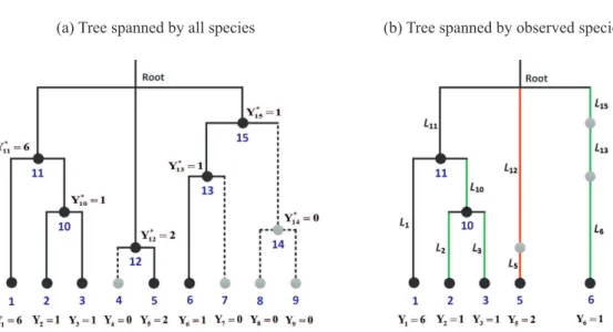
A rapidly growing literature discusses phylogenetic diversity, which incorporates evolutionary histories among species into diversity analysis (see Faith, 1992; Warwick and Clarke, 1995; Crozier, 1997; Webb and Nonoghue, 2005; Petchey and Gaston, 2002; Cadotte et al., 2009; Cavender-Bares, Ackerly and Kozak, 2012). The most widely used phylogenetic metric is Faith’s (1992)PD(phylogenetic diversity), which is defined as the sum of the branch lengths of a phylogenetic tree connecting all species in the target assemblage. As shown by Chao et al. (2010, 2015),PDcan be regarded as a measure of phylogenetic richness, i.e. a phylogenetic generalization of species richness. Through-out this paper, PD refers to Faith’s (1992) PD. When some species are present, but undetected by a sample, the lineages/branches associated with these undetected species are also missing from the phylogenetic tree spanned by the observed species. The unde-tectedPDin an incomplete sample was not discussed until recent years (Cardoso et al., 2014; Chao et al., 2015). In Section 6, we review the phylogenetic version of Chao’s

in-equality, developed recently by Chao et al. (2015), and the associated phylogenetic ver-sion of the rarefaction/extrapolation approach.

In Section 7, a small empirical dataset for Australian birds is used for illustration using online software, including Chao’s SpadeR, iNEXT, and PhD. Section 8 provides discussion and conclusions. The diversity measures discussed in this review (species richness, shared species richness, andPD) do not take species abundances into account. We briefly discuss the extension of these measures to incorporate species abundances, and refer readers to relevant papers. Major notation used in each section is shown in Table 1.

2. Species richness estimation

2.1. A general framework: Sampling-unit-based incidence data and model

As indicated in the Introduction, Chao’s (1987) original inequality was formulated based on a capture-recapture model to estimate the size of a population, but here we consider a framework based on species incidence (detection/non-detection) data to estimate species richness. These two statistical inference problems are equivalent. Assume that there are

Sspecies indexed 1,2, . . . ,Sin the focal assemblage, whereSis the estimating target in species richness estimation. Here we mainly consider the model developed by Colwell et al. (2012) for multiple incidence data. Assume that there areTsampling units, and that they are indexed 1,2, . . . ,T. The sampling unit is usually a trap, net, quadrat, plot, or timed survey, and it is these sampling units, not the individual organisms, that are sam-pled randomly and independently. The observed data consist of species detection/non-detection in each sampling unit. In a typical spatial study, these sampling units are deployed randomly in space within the area encompassing the assemblage. However, in a temporal study of diversity, theT sampling units would be deployed in one place at different independent points in time (such as an annual breeding bird census at a single site).

For any sampling unit, the model assumes that theith species has its own unique incidence or detection probabilityπi that is constant among all randomly selected sam-pling units. The incidence probabilityπiis the probability that speciesiis detected in a sampling unit. HerePS_i=1πiwill generally not be equal to unity.

The incidence records consist of a species-by-sampling-unit incidence matrix{Wi j;

i=1,2, . . . ,S, j=1,2, . . . ,T}withS rows andT columns; hereWi j=1 if speciesiis detected in sampling unit j, andWi j=0 otherwise. LetYi be the number of sampling units in which speciesiis detected,Yi=

PT

j=1Wi j; hereYi is referred to as the sample

species incidence frequency. Species present in the assemblage but not detected in any sampling unit yieldY =0. See Section 6.1 for a hypothetical example and Appendices A and B for real data. Details about these data are provided in subsequent sections.

8 Thirty years of progeny from Chao’s inequality: Estimating and comparing richness...

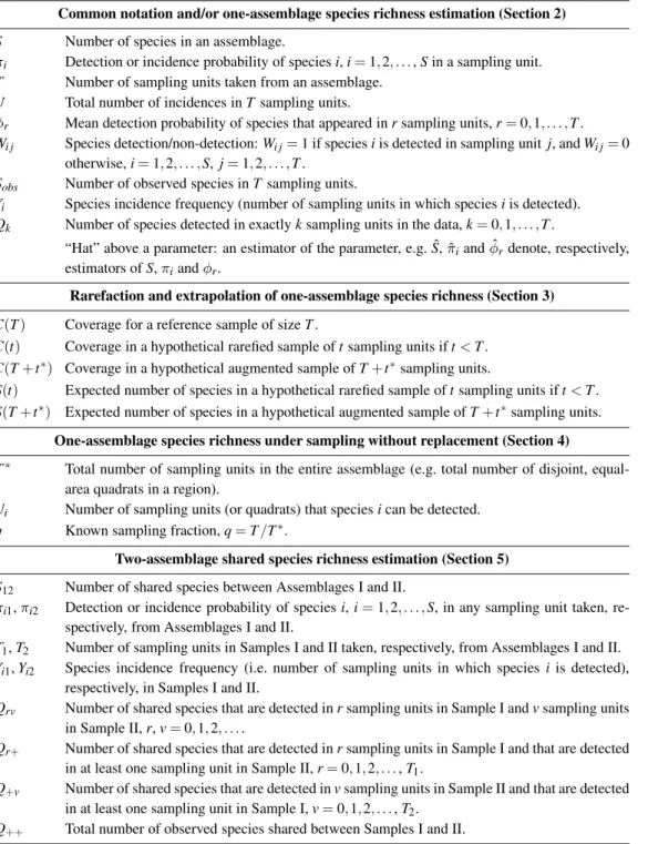
Table 1: Major notation used in each section.

Common notation and/or one-assemblage species richness estimation (Section 2)

S Number of species in an assemblage.

πi Detection or incidence probability of speciesi,i=1,2, . . .,Sin a sampling unit.

T Number of sampling units taken from an assemblage.

U Total number of incidences inT sampling units.

φr Mean detection probability of species that appeared inrsampling units,r=0,1, . . . ,T.

Wi j Species detection/non-detection:Wi j=1 if speciesiis detected in sampling unitj, andWi j=0 otherwise,i=1,2, . . . ,S, j=1,2, . . . ,T.

Sobs Number of observed species inT sampling units.

Yi Species incidence frequency (number of sampling units in which speciesiis detected).

Qk Number of species detected in exactlyksampling units in the data,k=0,1, . . . ,T.

ˆ “Hat” above a parameter: an estimator of the parameter, e.g. ˆS, ˆπiand ˆφrdenote, respectively, estimators ofS,πiandφr.

Rarefaction and extrapolation of one-assemblage species richness (Section 3)

C(T) Coverage for a reference sample of sizeT.

C(t) Coverage in a hypothetical rarefied sample oftsampling units ift<T.

C(T+t∗) Coverage in a hypothetical augmented sample ofT+t∗sampling units.

S(t) Expected number of species in a hypothetical rarefied sample oftsampling units ift<T.

S(T+t∗) Expected number of species in a hypothetical augmented sample ofT+t∗sampling units. One-assemblage species richness under sampling without replacement (Section 4)

T∗ Total number of sampling units in the entire assemblage (e.g. total number of disjoint, equal-area quadrats in a region).

Ui Number of sampling units (or quadrats) that speciesican be detected.

q Known sampling fraction,q=T/T∗.

Two-assemblage shared species richness estimation (Section 5)

S12 Number of shared species between Assemblages I and II.

πi1,πi2 Detection or incidence probability of speciesi,i=1,2, . . . ,S, in any sampling unit taken, re-spectively, from Assemblages I and II.

T1,T2 Number of sampling units in Samples I and II taken, respectively, from Assemblages I and II.

Yi1,Yi2 Species incidence frequency (i.e. number of sampling units in which species iis detected), respectively, in Samples I and II.

Qrv Number of shared species that are detected inrsampling units in Sample I andvsampling units in Sample II,r,v=0,1,2, . . ..

Qr+ Number of shared species that are detected inrsampling units in Sample I and that are detected in at least one sampling unit in Sample II,r=0,1,2, . . .,T1.

Q+v Number of shared species that are detected invsampling units in Sample II and that are detected in at least one sampling unit in Sample I,v=0,1,2, . . .,T2.

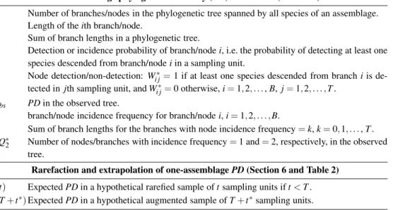
Table 1 (cont.): Major notation used in each section.

One-assemblage phylogenetic diversity (PD) Estimation (Section 6)

B Number of branches/nodes in the phylogenetic tree spanned by all species of an assemblage.

Li Length of theith branch/node.

PD Sum of branch lengths in a phylogenetic tree.

λi Detection or incidence probability of branch/nodei, i.e. the probability of detecting at least one species descended from branch/nodeiin a sampling unit.

W_{i j}∗ Node detection/non-detection: W_{i j}∗=1 if at least one species descended from branchiis de-tected in jth sampling unit, andW_{i j}∗=0 otherwise,i=1,2, . . .,B, j=1,2, . . . ,T.

PDobs PDin the observed tree.

Y_i∗ branch/node incidence frequency for branch/nodei,i=1,2, . . . ,B.

Rk Sum of branch lengths for the branches with node incidence frequency=k,k=0,1, . . .,T.

Q∗₁,Q∗₂ Number of nodes/branches with incidence frequency=1 and=2, respectively, in the observed tree.

Rarefaction and extrapolation of one-assemblagePD(Section 6 and Table 2)

PD(t) ExpectedPDin a hypothetical rarefied sample oftsampling units ift<T.

PD(T+t∗)ExpectedPDin a hypothetical augmented sample ofT+t∗sampling units.

Following Colwell et al. (2012), we assume, given the set of detection probabilities (π1, π2, . . . , πS), that each elementWi j in the incidence matrix is a Bernoulli random variable with probabilityπi. The probability distribution for the incidence matrix can be expressed as P(Wi j=wi j;i=1,2, . . . ,S, j=1,2, . . . ,T) = T

∏

∏

∏

P(Yi=yi) = T yi πyi i (1−πi) T−yi_{, i=1,2, . . . ,S. (1b)} Denote theincidence frequency countsby(Q1,Q2, . . . ,QT), whereQkis the number of species detected in exactlyk sampling units in the data,k =0,1, . . . ,T. Here, Q1 represents the number of “unique” species (those that are detected in only one sampling unit), andQ2 represents the number of “duplicate” species (those that are detected in exactly two sampling units). The unobservable zero frequency countQ0 denotes the number of species among theSspecies present in the assemblage that are not detected in any of theT sampling units. Then the number of observed species in the sample is

Sobs= P

10 Thirty years of progeny from Chao’s inequality: Estimating and comparing richness...

2.2. Chao’s inequality

Treating the incidence probabilities (π1, π2, . . . , πS) as fixed, unknown parameters, we first present Chao’s (1987) inequality under the model (1a) or (1b). Note the following expected value for the incidence frequency countQk:

E(Qk) =E " _S X i=1 I(Yi=k) # = S X i=1 T k πki(1−πi) T−k , k=0,1,2, . . . ,T, (1c) whereI(A)is the indicator function, i.e.I(A) =1 if the eventAoccurs, and is 0 other-wise. In particular, the expected number of undetected species, uniques and duplicates are respectively: E(Q0) = S X i=1 (1−πi)T_, E(Q1) = S X i=1 Tπi(1−πi)T−1_, E(Q2) = S X i=1 T 2 π2 i(1−πi) T−2_.

Chao (1987) proposed a lower bound ofE(Q0)based on the following Cauchy-Schwarz inequality: " _S X i=1 (1−πi)T # " _S X i=1 π2i(1−πi) T−2 # ≥ " _S X i=1 πi(1−πi)T−1 #2 , (2a) equivalently, E(Q0)× E(Q2) T 2 ≥ E(Q1) T 2 .

Thus, a theoretical lower bound forE(Q0)is derived as

E(Q0)≥ (T−1) T [E(Q1)]2 2E(Q2) ,

implying a theoretical lower bound for species richness:

S=E(Sobs) +E(Q0)≥E(Sobs) + (T−1) T [E(Q1)]2 2E(Q2) .

Replacing the expected values in the above with the observed data, we then obtain an estimated lower bound of species richness, with a slight modification when Q2 =0 (Colwell and Coddington, 1994, gave the nameChao2 to this estimator):

ˆ SChao2=          Sobs+ (T−1) T Q2 1 2Q2 , ifQ2>0, Sobs+ (T−1) T Q1(Q1−1) 2 , ifQ2=0. (2b)

The estimated number of undetected species is based exclusively on the information on the least frequent species (the number of uniques and duplicates). This is based on a basic concept that the frequent/abundant species (those that occur in many sampling units) carry negligible information about the undetected species; only rare/infrequent species carry such information.

When does the Chao2 formula provide a nearly unbiased estimator? The Cauchy-Schwarz inequality in Eq. (2a) becomes an equality if and only if the species detection probabilities are homogeneous, that is,π1=π2=· · ·=πS. Homogeneity of detection probabilities would be a very restrictive condition, one that is almost never satisfied in most practical applications, such as species abundance or incidence distributions in nature. However, as we will show in Section 2.3, this condition can be considerably re-laxed from a different derivation/perspective. Note that in Chao’s inequality (2a), only three expected frequency counts are involved:E(Q0),E(Q1)andE(Q2). The frequent species (species with relatively large detection probabilities) would tend to occur in many sampling units and thus generally do not contribute to any of these three terms. On the other hand, only rare/infrequent species (species with relatively low detection probabilities) would either be undetected or detected in only one or two sampling units and thus are those species that contribute to the three terms. Therefore, a relaxed condi-tion for an unbiased Chao2 estimator is thatvery rare/infrequentspecies have approx-imately the same detection probabilities, and frequent species are allowed to be highly heterogeneous without affecting the estimates. A more rigorous justification is given in Section 2.3.

Applying a standard asymptotic approach (Chao, 1987), the following estimated variance estimators can be obtained ifQ1,Q2>0:

c var(SˆChao2) =Q2 " 1 4 T−1 T 2 Q1 Q2 4 + T−1 T 2 Q1 Q2 3 +1 2 T−1 T Q1 Q2 2# , (3a) IfQ1>0,Q2=0, the variance becomes

c var(_Sˆ_{Chao2) =}1 4 T−1 T 2 Q1(2Q1−1)2+ 1 2 T−1 T Q1(Q1−1)− 1 4 T−1 T 2 Q4₁ ˆ SChao2 . (3b)

12 Thirty years of progeny from Chao’s inequality: Estimating and comparing richness...

In the special case thatQ1=0, we have ˆSChao2=Sobs, implying that sampling is complete and there are no undetected species in the data; an approximate variance of

Sobs can be obtained using an analytic method (Colwell, 2013) or a bootstrap method (see Section 3.3). WhenQ1>0 so that ˆSChao2>Sobs, the distribution of ˆSChao2−Sobsis generally skewed to the right. Using a log-transformation by treating log(_Sˆ_{Chao2−Sobs)} as an approximately normal random variable, we obtain a 95% confidence interval for

S: (Chao, 1987)

[Sobs+ (SˆChao2−Sobs)/R, Sobs+ (SˆChao2−Sobs)R], (3c) whereR=exp{1.96[log(1+varc(SˆChao2)/(SˆChao2−Sobs)2)]1/2}. In this case, the result-ing lower confidence limit is always greater than or equal to the observed species rich-ness, a sensible result.

The Chao2 estimator is also valid in a binomial-mixture model in which incidence probabilities (π1, π2, . . . , πS)are assumed to be a random sample from an unknown dis-tribution with densityh(π). Under this model, we have

E(Qk) =S 1 Z 0 T k πk(1−π)T−kh(π)dπ, k=0,1,2, . . .T. (4a)

The summation terms in the Cauchy-Schwarz inequality (2a) are replaced by integral terms:   1 Z 0 (1−π)Th(π)dπ     1 Z 0 π2(1−π)T−2h(π)dπ  ≥   1 Z 0 π(1−π)T−1h(π)dπ   2 . (4b)

The above two formulas also lead to the same Chao2 formula given in Eq. (2b). In the special case thath(π)is a beta distribution with parametersα andβ, the resulting expected incidence-frequency count{E(Qk),k=0,1,2, . . . ,n}correspond to the prob-abilities of a beta-binomial distribution. Under the two conditions (i)T is large and π

is small, such thatTπ tends to a positive constant, and (ii)β/T tends to a positive con-stantc, Skellam (1948) proved thatE(Qk) tends to(α+k−1)![(α−1)!k!]−1_[1/(1+

c)]k_[c/(1+c)]α

, which is the probability of a negative binomial variable taking the valuek. This result theoretically justifies the inference that Chao’s inequality is also valid for binomial and negative binomial distributions. It is well known that beta-binomial and negative beta-binomial can be used to describe spatially clustered (if sampling units are quadrats in an area) or temporally aggregated (if sampling units are differ-ent times) pattern of species; see Hughes and Madden (1993) and Shiyomi, Takahashi and Yoshimura (2000). Therefore, even though there is spatial/temporal heterogeneity pattern for species incidences, the lower bound and the associated estimation are still valid.

2.3. When is the Chao2 estimator nearly unbiased?

Alan Turing and I. J. Good, in their famous cryptanalysis to crack German ciphers dur-ing World War II, developed novel statistical methods to estimate the true frequencies of rare code elements (including still-undetected code elements), based on the observed frequencies in “samples” of intercepted Nazi code. After the War, Turing gave per-mission to Good to publish their statistical work. An influential paper by Good (1953) and one by Good and Toulmin (1956) presented Turing’s wartime statistical work on the frequency formula and related topics; see Good (1983, 2000) for more details. The frequency formula is now referred to as the Good-Turing frequency formula, which has a wide range of applications in biological sciences, statistics, computer sciences, infor-mation sciences, and linguistics, among others (McGrayne, 2011, p. 100).

In an ecological context, Turing’s statistical problem can be formulated as an esti-mation of the true frequencies of rare species when a random sample of individuals is drawn from an assemblage. In Turing’s case, there were almost infinitely many rare species so that all samples have undetected species. The Good-Turing formula answers the following question: given a species that appearsrtimes (r=0,1,2, . . .) in a sample ofnindividuals that fails to detect all species present, what is its true relative frequency in the entire assemblage? Turing and Good focussed on the case of small r, i.e. rare species. Turing gave a surprisingly simple and remarkably effective answer that is con-trary to most people’s intuition; see Chao et al. (2017) for a review.

The Good-Turing original frequency formula was based on abundance data. We here extend their formula to incidence data to answer the following question: Given species incidence data ofT sampling units, for those species that appeared inr (r=0,1,2, . . .) out ofT sampling units, what is the mean detection probability of species that appeared inr sampling units,φr? Such a mean detection probability can be mathematically ex-pressed as φr= S X i=1 πiI(Yi=r)/Qr, r=0,1,2, . . . (5a) The numerator in Eq. (5a) represents the total incidence probabilities of those species that appeared inrsampling units. Dividing the total byQr, we obtain the mean detection probability per species, among those that each appeared inr sampling units. Note that, for the special case ofr=0, Eq. (5a) implies

φ0Q0= S X

i=1

πiI(Yi=0), (5b) which is the total detection probabilities of the undetected species. If one additional sampling unit can be added, then we can interpret it as the expected number of species in the additional sampling unit that are undetected in the original sample.

Here we derive the corresponding Good-Turing incidence frequency formula for multiple incidence data by treating (π1, π2, . . . , πS) as fixed, unknown parameters,

al-14 Thirty years of progeny from Chao’s inequality: Estimating and comparing richness...

though a similar derivation is also valid for binomial-mixture models. Under the model (Eq. 1b), in which the incidence frequenciesYi,i=1,2, . . . ,S, follow a binomial distri-bution characterized byT and detection probabilityπi, we can express the sum of the odds ofπifor those species that each appeared inrsampling units as follows:

E " _S X i=1 πi 1−πi I(Yi=r) # = S X i=1 πi 1−πi T r πr i(1−πi) T−r = S X i=1 T r πr+1 i (1−πi) T−(r+1) = T r T r+1 " _S X i=1 T r+1 πr+1 i (1−πi) T−(r+1) # = (r+1) (T−r)E(Qr+1). (5c)

Assume that all species that appeared inrsampling units have approximately the same incidence probabilities. Then we have the following approximation formula:

E " _S X i=1 πi 1−πi I(Yi=r) # ≈Qr φr 1−φr .

Thus,φrcan be obtained by solving the equation:Qrφr/(1−φr)≈(r+1)Qr+1/(T−r), based on Eq. (5c). We then obtain the corresponding Good-Turing formula for incidence data: ˆ φr= (r+1)Qr+1 (T−r)Qr+ (r+1)Qr+1 ≈(r+1)Qr+1 (T−r)Qr . (5d) The original Good-Turing frequency formula for abundance data has a similar form as the above approximation, but with incidence frequency counts being replaced by abundance frequency counts.

Good (1983, p. 28) provided an intuitive justification for the abundance-based Good-Turing frequency formula. Here we follow Good’s approach to give a similar justifica-tion for incidence data. Given an original sample, consisting ofT sampling units, sup-pose one additional sampling unit can be added. We ask how many species that had ap-pearedrtimes in the original sample would occur in the additional sampling unit. Based on Eq. (5a), the answer is simplyPS_i=1πiI(Yi=r) =φrQr, which can be estimated by (r+1)Qr+1/(T−r)using the following simple reasoning. Notice that any species that appearedr times in the original sample and also occurs in the additional sampling unit

must occur inr+1 sampling units in the enlarged sample consisting ofT+1 sampling units. Then the total number of incidences of such species is (r+1)Qr+1. Because the order in which sampling units were taken is assumed to be irrelevant, the average number of such species occurring in a single sampling unit is thus(r+1)Qr+1/(T+1), which is approximately equal to(r+1)Qr+1/(T−r)ifr is small. Dividing this ratio by the number of such species,Qr, we obtain the incidence-data-based Good-Turing frequency formula forφras given in Eq. (5d).

For the special cases ofr=0 andr=1, Eqs. (5b) and (5d) lead to [ φ0Q0= Q1 T ,φˆ1= 2Q2 (T−1)Q1 ,

whereφ[0Q0 denotes the estimate of the product of φ0 and Q0. Intuitively, we expect that the mean incidence probability of all undetected species should not be more than that of all uniques in the sample, i.e. φ0 ≤φ1, and this ordering is preserved by the corresponding estimates. Then we obtain the Chao2 lower bound for the number of undetected species by the following inequality:

ˆ Q0= [ φ0Q0 ˆ φ0 ≥φ[0Q0 ˆ φ1 = Q₁ T 2Q2 (T−1)Q₁ = (T−1) T Q2₁ 2Q2 . (5e)

Notice that, in the above derivation, if ˆφ0≈φˆ1, then the inequality sign in Eq. (5e) becomes an equality sign. Therefore, from the Good-Turing perspective, the Chao2 lower bound is a nearly unbiased point estimator if all undetected and unique species in samples have the same mean detection probabilities. Such a conclusion is valid if very rare/infrequent species have approximately homogenous detection probabilities in any sampling unit (because this implies ˆφ0 ≈φˆ1); in this case, frequent species could be highly heterogeneous without affecting the estimator.

2.4. How many sampling units are needed to reach the Chao2 estimate?

As discussed earlier, the Chao2 formula (in Eq. 2b) implies that sampling is complete when all species have been found in at least two sampling units, i.e.Q1=0; in such a case, the estimated undetected species richness is 0 and the estimated species rich-ness reduces simply to the observed number of species. This result also reveals that, whenever at least one species is found in only one sample (Q1>0), sampling is not complete and some species remain undetected. However, the Chao2 species richness estimator does not indicate how much sampling effort (how many additional sampling units) would be necessary to reach the Chao2 estimate (i.e. the first point at which there are no longer any singletons).

For incidence data, “sample size” means the number of sampling units. Chao et al. (2009) developed a non-parametric method for estimating the minimum sample size

16 Thirty years of progeny from Chao’s inequality: Estimating and comparing richness...

required to detect any arbitrary proportion (including 100%) of the estimated Chao2 species richness based on the Good-Turing formula discussed in Section 2.3. When the target is the Chao2 estimate, Chao et al. (2009) approach is to predict the minimum sample sizetto achieve the following stopping rule: there are no uniques in the enlarged sample of sizeT+t, or equivalently, the expected number of uniques in the enlarged sample of sizeT+tis less than 0.5, because the theoretical expected value may not be an integer.

Note that the number of uniques in the enlarged sample of sizeT+tincludes two groups of species: (1) any species observed in only one sampling unit in the original sample (i.e. those species withYi=1) for which no additional incidences are detected in the additionaltsamples with probability (1−πi)t_{, and (2) any species not detected} in the original sample (i.e. those species withYi=0) for which detection in exactly one sampling unit is observed in the additionalt sampling units with probabilitytπi(1−

πi)t−1_{. That is, the expected number of uniques in the enlargedT+tsampling units is:} XS i=1(1−πi) t I(Yi=1) + XS i=1tπi(1−πi) t−1_I(Y i=0).

As discussed in Section 2.3, we assume that all uniques in the original sample have mean detection probabilityφ1, and all previously undetected species have mean detec-tion probabilityφ0. Then the number of uniques in the enlargedT+t sampling units will decline to<0.5 whentsatisfies

Q1(1−φ1)t+Q0tφ0(1−φ0)t−1<0.5.

When we apply the Good-Turing incidence frequency formula to this equation, and substitute φ1, φ0 and Q0 by ˆφ1 =2Q2/[2Q2+ (T −1)Q1], ˆφ0 =Q1/[Q1+TQˆ0] and

ˆ

Q0= (1−1/T)Q12/(2Q2), then the requiredtmust satisfy the following equation:

Q1 1+ t T 1− 2Q2 (T−1)Q1+2Q2 t <0.5.

The additional number of sampling units needed to reach the Chao2 estimate is approx-imately equal tot=T x∗, wherex∗is the solution of the following equation:

2Q1(1+x) =exp x 2Q2 (1−1/T)Q1+2Q2/T . (6a) Ifgis the fraction of ˆSChao2 that is desired (0<g<1), then the objective is to find the number of additionalmg sampling units such that the number of species reaches the target valuegSˆChao2, i.e. the expected number of previously undetected species that will be discovered in the additionalmgsampling units isgSˆChao2−Sobs. This expected number, given the observed data, is

S X

i=1

[1−(1−πi)mg_]I(Y

i=0)≈Q0[1−(1−φ0)mg]. (6b) Applying the Good-Turing incidence frequency formula and substituting φ0 and Q0, we obtain that the required number of additional sampling units to reach a fractiongof

ˆ

SChao2(ifgSˆChao2>Sobs)is the numbermgsuch that ˆQ0[1−(1−φˆ0)mg] =gSˆChao2−Sobs, i.e. mg≈ log 1− T (T−1) 2Q2 Q2 1 (gSˆChao2−Sobs) log 1− 2Q2 (T−1)Q1+2Q2 . (6c)

Chao et al. (2009) also provided an Excel spreadsheet for calculating necessary sampling effort for either abundance data or replicated incidence data.

2.5. A class of lower bounds

In the Chao2 approach (Eq. 2b), the estimator for undetected species richness is only in terms of the species incidence frequency counts of the uniques and duplicates in data. Several authors extended this approach to higher-order incidence frequency counts. Lanumteang and B¨ohning (2011) proposed using an additional incidence frequency count, i.e. the number of species that are detected in exactly three sampling units. They applied the above estimator to a variety of real data sets and concluded that the new estimator is especially useful for large populations and heterogeneous detection proba-bilities.

When the Chao2 estimator only provides a lower bound, its bias can be evaluated and assessed by using the Good-Turing frequency formula. In this case, an improved reduced-bias lower bound, which makes use of the additional information ofQ3andQ4, was derived by Chiu et al. (2014). The corresponding lower bound of species richness is referred to asiChao2 estimator(here the sub-indexistands for “improved”):

ˆ SiChao2=SˆChao2+ (T−3) 4T Q3 Q4 ×max Q1− (T−3) 2(T−1) Q2Q3 Q4 ,0 . (6d) They also provided an analytic variance estimator to construct the associated confidence intervals.

Puig and Kokonendji (2017) extended Chao’s inequality to a broader class of distri-butions that have log-convex probability generating functions. They obtained a series of lower bounds for the undetected species richness. This class of distribution includes compound Poisson distribution and Poisson-mixture distributions. Their framework is mainly based on abundance data, but it can be readily applied to multiple incidence data, as shown below.

18 Thirty years of progeny from Chao’s inequality: Estimating and comparing richness...

Following the proof of Puig and Kokonendji (2017), we assume that the incidence probabilities (π1, π2, . . . , πS) are a random sample from an unknown distribution with densityh(π), and we haveE(Qk) given in Eq. (4a). Consider a probability density function: H(π) = (1−π) T_h(π)dπ R1 0 (1−u)Th(u)du , 0< π <1.

Puig and Kokonendji (2017) showed the following moment inequality forr,v=0,1,2, . . .

1 Z 0 π 1−π r+v H(π)dπ≥ 1 Z 0 π 1−π r H(π)dπ× 1 Z 0 π 1−π v H(π)dπ, equivalently,   1 Z 0 (1−π)T_h(π)dπ     1 Z 0 πr+v_(1−π)T−(r+v)_h(π)dπ   ≥   1 Z 0 πr(1−π)T−rh(π)dπ     1 Z 0 πv(1−π)T−vh(π)dπ  . Then we have E(Q0)≥ T r+v E(Qr)×E(Qv) T r T v E(Qr+v) , r,v=0,1,2, . . . (6e)

A series of lower bounds ofScan then be obtained ifQr+v>0:

Sobs+ T r+v Qr×Qv T r T v Qr+v , r,v=1,2, . . .

In the special case ofr=v=1, the above lower bound reduces to the Chao2 estimator. Puig and Kokonendji (2017) proved that, under a Poisson-mixture model, the greatest lower bound attains at the special caser=v=1. This also provides a justification for the use of the Chao2 lower bound.

3. Species richness estimation for standardized samples:

non-asymptotic analysis

Species richness estimation represents an “asymptotic” analysis; here “asymptotic” means that, as sample size tends to infinity, sample completeness approaches unity. When the Chao2 estimates are nearly unbiased under the conditions given in Section 2.3, they can be compared across multiple assemblages. However, when rare/infrequent species are highly heterogeneous and sample size is not sufficiently large, the Chao2 formula can provide only a lower bound, which cannot be compared accurately across assemblages, because the data provide insufficient information to accurately estimate species richness due to high heterogeneity of infrequent species. No matter whether or not Chao2 is unbiased, in any particular case, we can always use it to perform “non-asymptotic” analysis, in which samples are standardized based on a common finite sample size or on sample completeness via rarefaction and extrapolation. Again for incidence data, sample size refers to the number of sampling units.

The objective of a non-asymptotic approach is to control the dependence of the em-pirical species counts on sampling effort and sample completeness. The earliest devel-opment of standardization of sample size for abundance data by rarefaction was pro-posed by Sanders (1968), but see Chiarucci et al. (2008) for a historical review. Subse-quent developments include studies by Hurlbert (1971), Simberloff (1972), Heck, van Belle and Simberloff (1975) and Coleman et al. (1982); see Gotelli and Colwell (2001, 2011) for details. Ecologists typically use rarefaction to down-sample the larger sam-ples until they are the same size as the smallest sample. Ecologists then compare rich-ness of these equally-large samples, but this approach implies that some data in larger samples are thrown away. To avoid discarding data, Colwell et al. (2012) proposed using a unified sample-size-based rarefaction (interpolation) and extrapolation (predic-tion) sampling curve for species richness, that can be rarefied to smaller sample sizes or extrapolated to larger sample sizes.

Chao and Jost (2012) indicated that a sample of a given size may be sufficient to fully characterize a low-diversity assemblage, but insufficient to characterize a rich-assemblage. Thus, when the species counts of two equally-large samples are compared, one might be comparing a nearly complete sample to a very incomplete one. In this case, any difference in diversity between the sites will generally be underestimated. They pro-posed rarefaction and extrapolation to a comparable degree of sample completeness (as measured by sample coverage; see below) and developed a coverage-based rarefaction and extrapolation methodology. The sample-size-based and coverage-based integration of rarefaction and extrapolation of species richness represent a unified sampling frame-work for quantifying and comparing species richness across multiple assemblages.

Here we review the sample-size-based and coverage-based rarefaction and extrapo-lation of species richness; all formulas are tabulated in the first and the third columns of Table 2.

2 0 T h ir ty y e a rs o f p ro g e n y fro m C h a o ’s in e q u a lit y : E s tim a tin g a n d c o m p a rin g ric h n e s s ...

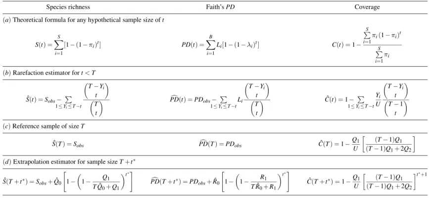
Table 2: The theoretical formulas and analytic estimators for rarefaction and extrapolation of species richness (left column), Faith’s PD (middle column), and sample coverage (right column) based on incidence data, given a reference sample with observed species richness=Sobs, observed PD=PDobs, and estimated coverageC(Tˆ )for incidence data. Here the sample size means the number of sampling units. See Colwell et al. (2012) and Chao and Jost (2012) for derivation details.

Species richness Faith’sPD Coverage

(a)Theoretical formula for any hypothetical sample size oft

S(t) = S X i=1 [1−(1−πi)t] PD(t) = B X i=1 Li[1−(1−λi)t] C(t) =1− S P i=1 πi(1−πi)t S P i=1 πi (b)Rarefaction estimator fort<T

ˆ S(t) =Sobs− P 1≤Yi≤T−t T−Yi t T t PD(t) =c PDobs− P 1≤Yi≤T−t Li T−Yi t T t _{C(t) =}ˆ ₁₋ P 1≤Yi≤T−t Yi U T−Yi t T−1 t

(c)Reference sample of sizeT ˆ S(T) =Sobs PD(Tc ) =PDobs C(Tˆ ) =1− Q1 U _(T−1)Q 1 (T−1)Q1+2Q2

(d)Extrapolation estimator for sample sizeT+t∗ ˆ S(T+t∗) =Sobs+Qˆ0 " 1− 1− Q1 TQˆ0+Q1 t∗# c PD(T+t∗) =PDobs+Rˆ0 " 1− 1− R1 TRˆ0+R1 t∗# ˆ C(T+t∗) =1−Q1 U _(T−1)Q 1 (T−1)Q1+2Q2 t∗₊₁

Notes:U=P_Yi>0Yi=PTj=1jQjdenotes the total number of incidences inT sampling units; ˆQ0and ˆR0denote the estimated number of undetected species

3.1. Sample-size-based rarefaction and extrapolation

Following Colwell et al. (2012), we refer to the observed sample ofT sampling units as areference sample. Let S(t) be the expected number of species in a hypothetical sample oft sampling units, randomly selected from the sampling units that represent the assemblage. If we knew the true species detection probabilities (π1, π2, . . . , πS) of theSspecies in each sampling unit, we could compute the following expected value:

S(t) =S− S X

i=1

(1−πi)t, t=1,2, . . . (7a) The plot ofS(t) with respect to the number of sampling units t is the sampling-unit-based species accumulation curve. Note that the true species richness represents the “asymptote” of the curve, i.e.S=S(∞). The rarefaction (interpolation) part estimates the expected species richness for a smaller number of sampling unitst<T. On the basis of a reference sample ofT sampling units, an unbiased estimator ˆS(t)forS(t),t<T, is

ˆ S(t) =Sobs− X 1≤Yi≤T−t T−Yi t , T t , t<T. (7b) This analytic formula was first derived by Shinozaki (1963) and rediscovered multiple times (Chiarucci et al., 2008).

The extrapolation is to estimate the expected number of speciesS(T+t∗)in a hypo-thetical sample ofT+t∗sampling units (t∗>0) from the assemblage. Rewrite

S(T+t∗) = S X i=1 [1−(1−πi)T+t∗_] = S X i=1 [1−(1−πi)T_{] +} S X i=1 [1−(1−πi)t∗_](1−πi)T =E(Sobs) +E " _S X i=1 [1−(1−πi)t∗_] I(Yi=0) # .

The first term in the above formula represents the observed species richness. For the second term, we can apply the Good-Turing incidence frequency formula (Section 2.3) by assuming that all previously undetected species have mean detection probabilityφ0. Then for the second term, we have

S X i=1 [1−(1−πi)t∗_]I(Y i=0)≈Q0[1−(1−φ0)t ∗ ].

22 Thirty years of progeny from Chao’s inequality: Estimating and comparing richness...

Based on Eq. (5d), we have the extrapolated species richness for a sample of sizeT+t∗: ˆ S(T+t∗) =Sobs+Qˆ0 " 1− 1− Q1 TQˆ0+Q1 t∗# , t∗≥0. (7c) Colwell et al. (2012) linked rarefaction and extrapolation to form an integrated smooth curve. The integrated sample-size-based sampling curve includes a rarefaction part (which plots ˆS(t)as a function oft<T), and an extrapolation part (which plots ˆS(T+t∗) as a function ofT+t∗), joining smoothly at the reference point (T,Sobs). The confidence intervals based on the bootstrap method (Section 3.3) also join smoothly.

For a short-range prediction (e.g. t∗ is much less than T), the extrapolation for-mula is independent of the choice of ˆQ0 as indicated by the approximation formula

ˆ

S(T+t∗)≈Sobs+ (Q1/T)t∗. This implies that the extrapolation formula in Eq. (7c) is very robust and reliable even though the species richness estimator is subject to bias. Previous experiences by Colwell et al. (2012) suggested that the prediction size can be extrapolated at most to double the observed sample size.

3.2. Coverage-based rarefaction and extrapolation

Turing and Good developed the very important concept of “sample coverage” to charac-terize the sample completeness of an observed set of individual-based abundance data. Their concept was extended by Chao et al. (1992) to capture-recapture data. For mul-tiple incidence data, thesample coverageof a reference sample ofT sampling units is defined as C≡C(T) = PS i=1πiI(Yi>0) PS i=1πi =1− PS i=1πiI(Yi=0) PS i=1πi ,

which represents the fraction of the total incidence probabilities in the assemblage (in-cluding undetected species) that is represented by species detected in the reference sam-ple. Note that under the binomial model (Eq. 1b), an unbiased estimator for the de-nominator inC(T)isU/T, whereU=PT_k=1kQk=

PS

i=1Yidenotes the total number of incidences in the reference sample. For the numerator, we can apply the Good-Turing incidence frequency formula (Section 2.3) by assuming that all uniques in the sample have approximately the same detection probabilities,φ1. Then we can write

EXS i=1πiI(Yi=0) =XS i=1πi(1−πi) T = 1 TE XS i=1(1−πi)I(Yi=1) ≈E(Q1) T (1−φ1).

Applying the Good-Turing formula ˆφ1=2Q2/[2Q2+ (T−1)Q1](Eq. 5d), we obtain a very accurate estimator of the sample coverage for the reference sample size, ifQ2>0:

ˆ C(T) =1−Q1 U (T−1)Q1 (T−1)Q1+2Q2 . (7d) IfQ2=0, a modified formula based on Chao et al. (2014b, Appendix G) is:

ˆ C(T) =1−Q1 U (T−1)(Q1−1) (T−1)(Q1−1) +2 . (7e) In addition to the reference sample, we also need to consider the estimation of the expected sample coverage, E[C(t)], for any hypothetical sample oft sampling units,

t=1,2, . . .. This expected sample coverage is a function oftas given below:

E[C(t)] =1− PS i=1πi(1−πi)t PS i=1πi , t≥1. (7f) For a rarefied sample (t<T), an unbiased estimator exists for the denominator and numerator in Eq. (7f), respectively, but their ratio ˆC(t), given below, is only a nearly unbiased estimator ofE[C(t)]: ˆ C(t) =1− X 1≤Y_i≤T−t Yi U T−Yi t T−1 t , t<T.

An estimator for the expected coverage of an extrapolated sample withT+t∗sampling units ifQ2>0 is ˆ C(T+t∗) =1−Q1 U (T−1)Q1 (T−1)Q1+2Q2 t∗+1 . (7g) The above estimator is based on the following approximation formula:

E[C(T+t∗)] =1− PS i=1πi(1−πi)T+t ∗ PS i=1πi ≈1−E[ PS i=1(1−πi)t ∗₊₁ I(Yi=1)] T PS_i=1πi , ≈1−[E(Q1)](1−φ1) t∗+1 T PS_i=1πi .

ReplacingPS_i=1πiandφ1 with their respective estimators,U/T and ˆφ1=2Q2/[2Q2+ (T−1)Q1], we obtain Eq. (7g). If Q2=0, a similar modification as in Eq. (7e) can be applied. Note that whent∗=0, Eq. (7g) reduces to the sample coverage estimator for the reference sample. The coverage-based sampling curve includes a rarefaction part (which plots ˆS(t) as a function of ˆC(t)), and an extrapolation part (which plots

ˆ

24 Thirty years of progeny from Chao’s inequality: Estimating and comparing richness...

( ˆC(T),Sobs). The confidence intervals based on the bootstrap method (Section 3.3) also join smoothly. To equalize coverage among multiple, independent reference samples, their coverage-based curves can be extended to the coverage of the maximum size used in the corresponding sample-size-based sampling curve.

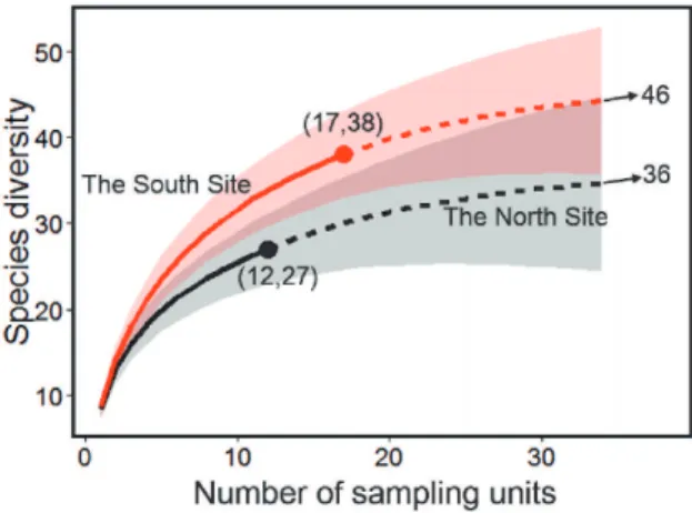
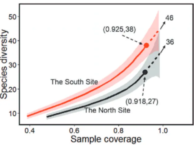
The sample-size-based approach plots the estimated species richness as a function of sample size, whereas the corresponding coverage-based approach plots the same rich-ness estimate with respect to sample coverage. Therefore, the two types of sampling curves can be bridged by a sample completeness curve, which shows how the sample coverage estimate varies with sample size and also provides an estimate of the sample size needed to achieve a fixed degree of completeness. The two types of sampling curves along with the associated sample completeness curve are illustrated in Section 7 through an example. There, we also illustrate the use of the online software iNEXT (iNterpola-tion/EXTrapolation) to compute and plot the integrated sampling curves for incidence data. These methods allow researchers to efficiently use all available data to make more robust and more detailed inferences about species richness of the sampled assemblages, and also to make objective comparisons of species richness across assemblages.

3.3. Bootstrap method to obtain variance estimator and confidence intervals

The interpolated and extrapolated estimators are complicated functions of incidence data. Thus, it is not possible to derive analytic variance estimators. A bootstrap pro-cedure can be applied to approximate the variance of any estimator based on incidence data. The estimated variance estimator can be subsequently used to construct a confi-dence interval of the expected species richness. Here we use the rarefied estimator ˆS(t) given in Eq. (7b) as an example. Parallel steps can be formulated for any extrapolated estimator, coverage estimators, and for Chao2-type estimators.

First, we construct thebootstrap assemblage, which aims to mimic the true entire as-semblage. Given a reference sample of sizeT and species sample incidence frequencies (Y1,Y2, . . . ,YS), let ˆQ0be the Chao2-type estimator of the number of undetected species. Since the number of species in the bootstrap assemblage must be an integer, we define

ˆ

Q∗₀ as the smallest integer that is greater than or equal to ˆQ0. Thus, there areSobs+Qˆ∗₀ species in the bootstrap assemblage.

Next we determine the detection probabilities in any sampling unit for the species in the bootstrap assemblage. Given that theith species is detected inYi >0 sampling units (there areSobs of such species), the sample detection probabilityYi/T of an ob-served species (Yi>0), on average, overestimates the true detection probabilityπi. This overestimation is due to the following conditional expectation:

E Yi T Yi>0 = πi 1−(1−πi)T > πi.

The above conditional expectation leads to πi=E Yi T Yi>0 [1−(1−πi)T_].

If we replace the expected value in the above equation by the observed data, then we have the following approximation:

πi≈

Yi

T[1−(1−πi)

T_{]. (7h)}

For any givenYi>1, one can numerically solve the above equation forπi; but forYi=1 (singletons, the most important count in our analysis), the only solution isπi=0, which is not reasonable. Therefore, Chao et al. (2014b, Appendix G) recommended the fol-lowing analytic approach. Note that Eq. (7h) reveals that the approximate adjustment factor for the sample detection probabilityYi/T would be[1−(1−πi)T]. However, the adjustment factor[1−(1−πi)T_{]cannot be estimated simply by substituting the sample} detection probability forπi, because the sample detection probability does not estimate

πiwell for rare species. Chao et al. (2014b) suggested a more flexible adjustment factor, [1−τ(1−Yi/T)T]. Applying this factor, we obtain that the species incidence probabili-ties for theSobsobserved species in the bootstrap assemblage can be estimated by

ˆ πi= Yi T " 1−τˆ 1−Yi T T# , Yi>0, (8a) where ˆτ can be obtained from the sample coverage estimate:

ˆ C(T)×U T = X i ˆ πiI(Yi>0) = X Yi>0 Yi T " 1−τˆ 1−Yi T T# ,

Then we can solve for ˆτ:

ˆ τ= U T[1−Cˆ(T)] P Y_i≥1 Yi T 1−Yi T T = [1−_Cˆ_(T)] P Y_i≥1 Yi U 1−Yi T T. (8b)

We assume that each of the remaining ˆQ∗₀ species in the bootstrap assemblage (i. e. those species that were not detected in any sampling unit but exist in the bootstrap assemblage) has a common detection probability of(U/T)[1−Cˆ(T)]/Qˆ∗₀. This assump-tion may seem restrictive, but the effect on the resulting variance estimator is limited, based on our extensive simulations.

After the bootstrap assemblage is determined, a random sample ofT sampling units is generated from the assemblage, and a bootstrap estimate ˆS(t) is calculated for the

26 Thirty years of progeny from Chao’s inequality: Estimating and comparing richness...

generated sample. The procedure is repeatedBtimes to obtainB bootstrap estimates (B=200 is suggested). The bootstrap variance estimator ˆS(t)is the sample variance of theseBestimates. The resulting bootstraps.e. of ˆS(t)is then used to construct a 95% confidence interval ˆS(t)±1.96s.e. [Sˆ(t)]for the expected species richness in a sample of sizet. Similar procedures can be used to derive variance estimators for any other estimator and its associated confidence intervals.

4. Species richness estimation under sampling without

replacement

Chao’s original inequality was developed under the binomial (Eq. 1b) model, which assumes that sampling units are taken with replacement. When sampling is done with-out replacement, e.g. quadrats or time periods that are not repeatedly selected/surveyed, or mobile species are collected by lethal sampling methods, Chao’s inequality and the Chao2 estimator require modification, unless the sampling fraction is small. For sim-plicity, we assume quadrat sampling in the following derivation, but the term “quadrat,” here, may refer to any sampling unit that is not sampled with replacement, such as a trap, net, team, observer, occasion, transect line, or fixed period of time in other sampling protocols. Suppose that the region under investigation consists ofT∗ disjoint, equal-area quadrats, and a sample of T quadrats is randomly selected. Then each quadrat is surveyed, and species detection/non-detection data are recorded for each of theseT

quadrats.

The model assumes that species i can be detected in only Ui quadrats (Ui is un-known). We restrict our analysis to the caseUi>1. (For any species withUi=0, there is no chance to detect this species in any sample, so it should be excluded from the es-timating target.) In the otherT∗−Uiquadrats, speciesiis either absent or it is present but cannot be detected. BecauseUi may vary independently among species, our model holds even if species are spatially aggregated, associated, or dissociated in the study area.

Assume that detection/non-detection of all species for each of the T quadrats is recorded to form a species-by-quadrat incidence matrix. Using the same notation as in Section 2, we letYi (sample incidence frequency) be the number of quadrats in which theith species is observed in the sample,i=1,2, . . . ,S. Under sampling without replacement, the sample frequencies(Y1,Y2, . . . ,YS) givenUi =ui, follow a product-hypergeometric distribution: P(Yi=yi,i=1,2, . . . ,S) = S

∏

is relatively small (i.e.T∗≫T), then equation (9a) approaches the product binomial distribution: P(Yi=yi,i=1,2, . . . ,S)→ S

∏

This is a model for sampling with replacement with incidence probabilitiesπi=ui/T∗. The above approximation shows that, if there are many quadrats, and only a small num-ber of the quadrats are sampled, then the inferences for the two types of sampling schemes differ little. Based on the general model (9a), the marginal distribution for each species’ frequency is a hypergeometric distribution. The expected value of the frequency counts is E(Qk) = S X i=1 P(Yi=k) = S X i=1 ui k T∗−ui T−k T∗ T . (9b) In particular, we have E(Q0) = S X i=1 T∗−ui T T∗ T , E(Q1) = S X i=1 ui 1 T∗−ui T−1 T∗ T = S X i=1 Tui T∗−ui−T+1 T∗−ui T T∗ T E(Q2) = S X i=1 ui 2 T∗−ui T−2 T∗ T = S X i=1 T(T−1)ui(ui−1) 2(T∗_−u i−T+1)(T∗−ui−T+2) T∗−ui T T∗ T

The Cauchy-Schwarz inequality leads to      S X i=1 T∗−ui T T∗ T           S X i=1 Tui T∗_−ui−T+1 2 T∗−ui T T∗ T     ≥      S X i=1 Tui T∗_−ui−T+1 T∗−ui T T∗ T      2 ,

The right side in the above inequality is{E(Q1)}2, and the first sum on the left side is