A Modified Membrane-Inspired Algorithm Based on Particle
Swarm Optimization for Mobile Robot Path Planning
X.Y. Wang, G.X. Zhang, J.B. Zhao, H.N. Rong, F. Ipate, R. Lefticaru
Xueyuan Wang
1. School of Electrical Engineering Southwest Jiaotong University Chengdu 610031, P.R. China
2. School of Information Engineering
Southwest University of Science and Technology MianYang 621010, P.R.China
Gexiang Zhang*, Junbo Zhao, Haina Rong
School of Electrical Engineering Southwest Jiaotong University Chengdu 610031, P.R. China
[email protected], [email protected], [email protected] *Corresponding author
Florentin Ipate, Raluca Lefticaru
Faculty of Mathematics and Computer Science University of Bucharest
Academiei 14, Bucharest, Romania
[email protected], [email protected]
Abstract
To solve the multi-objective mobile robot path planning in a dangerous environment with dynamic obstacles, this paper proposes a modified membrane-inspired algorithm based on particle swarm optimization (mMPSO), which combines membrane systems with particle swarm optimization. In mMPSO, a dynamic double one-level membrane structure is intro-duced to arrange the particles with various dimensions and perform the communications between particles in different membranes; a point repair algorithm is presented to change an infeasible path into a feasible path; a smoothness algorithm is proposed to remove the redundant information of a feasible path; inspired by the idea of tightening the fishing line, a moving direction adjustment for each node of a path is introduced to enhance the algorithm performance. Extensive experiments conducted in different environments with three kinds of grid models and five kinds of obstacles show the effectiveness and practicality of mMPSO.
Keywords: Membrane computing, evolutionary membrane computing, particle swarm optimization, variable dimensions, mobile robot path planning, membrane systems.
1
Introduction
As a branch of natural computing, membrane computing(MC), initiated by P˘aun in 1998, aims to abstract distributed and parallel computing models, also called P systems or membrane systems, from the compartmentalized structure and interactions of living cells [1, 2]. There are three main research directions in this area [3]: theoretical study including computing models
and their computing power and efficiency; applications such as modeling biological processes and approximately solving engineering optimization problems [4]; software and hardware realization. In the past fifteen years, much attention has been paid to the theoretical aspects, but the applications are worth further discussing, especially for solving real-world engineering problems. Evolutionary algorithms (EAs) are a class of probabilistic search methods with many advan-tages such as flexibility, convenient application and robustness. While MC can provide flexible evolution rules and parallel-distributed framework [5], which is very beneficial to produce the membrane-inspired evolutionary algorithms (MIEAs). Until now, different kinds of MIEAs have been proposed. In [6], a certain number of nested membrane structures in the skin membrane were combined with EAs for multi-objective optimization problems. A novel MIEA, called QEPS, combining quantum-inspired evolutionary algorithms with P systems to solve image pro-cessing problems and knapsack problems were proposed in [7, 8]. Particle swarm optimization (PSO) [9] with one-level membrane structure (OLMS) was used to solve broadcasting problems of P systems and radio spectrum allocation, respectively [10, 13]. In [11], Xiao et al. applied the bio-inspired algorithm based on membrane computing for engineering design problems.
These investigations prove the usefulness of introducing the P systems into EAs in order to solve various real-world applications. To the best of our knowledge, there is not any work focusing on the use of a MIEA to solve mobile robot path planning problems (MR3P), which is a very important real-world application.
In this paper, a modified membrane-inspired algorithm based on particle swarm optimization (mMPSO) is proposed to solve MR3P. The main contributions of this paper can be summarized as follows: (1) In this study, the solution to MR3P is considered as a dimension-reducing op-timization problem and therefore a PSO with variable dimensions (vPSO) is introduced into mMPSO, and further a dynamic double OLMS (D-OLMS) with membrane division and dis-solution is presented; this is combined with vPSO to arrange the particles and execute the communications between regions delimited by membranes. (2) Mobile robot path planning is a multi-objective optimization problem. This study considers three objectives, distance,safety
andsmoothness, instead of a single objective (path length) [15–17] or bi-objectives (path length and risk degree) as previously considered in the literature [18, 21]. A point repair algorithm and a smoothness approach are presented to effectively trade-off multiple objectives and speed-up the mMPSO convergence. (3) Inspired by the idea of tightening the fishing line, a moving di-rection adjustment for each node of a path is introduced to enhance the algorithm performance, together with the point repair algorithm. (4) Extensive experiments are carried out by con-sidering various environments with different grid models and different obstacles to verify the effectiveness and practicality of mMPSO.
The rest of this paper is organized as follows. Section 2 describes MR3P. In Section 3, we present mMPSO for solving MR3P. Section 4 discusses parameter setting and provides experi-mental results. Conclusions are drawn in Section 5.
2
Mobile Robot Path Planning Problems
This section gives a brief description of MR3P and then summarizes the related works.
2.1 Problem Statement
MR3P aims to find a reasonable collision-free path for a mobile robot from the starting position to the target position through an environment containing static or dynamic obstacles. It is proved that MR3P is an NP-complete problem [19]. Mobile robots are very useful for dangerous or hostile environments that humans are not able to reach. As one of the important
research themes in the mobile robotics field, MR3P, launched in the 1960s, has become an attractive and important research area.
Generally, the criterion for planning a mobile path has to consider many factors, such as the shortest distance, safety degree, smoothness, the lowest energy cost and minimum time, based on the characteristics of a special robot with the minimal turning radius, acceleration and the limited velocity and the features of the environment, such as the distances between obstacles, the shapes of obstacles, the occurrence probabilities of dynamic obstacles. Thus, the optimization of a mobile robot path in a static or dynamic environment is very complicated. For implementing the real time robot path planning in a dynamic environment or for dynamically tracking the motion target of a robot, at least three aspects should be carefully considered. These are also strongly interconnected.
(I) An efficient and effective optimization approach is very important for planning a good mobile robot path. Aiming to solve MR3P in a dynamic environment, this study proposes mMPSO.
(II) A simple and good objective function is very important for planning a good mobile robot path. In this study, the objective function aims to minimize the path length, to maximize the smoothness and the distances between a robot and the obstacles or dangerous sources, and can be expressed as
f =Kd·Dis+Kf ·S+Ks·SD (1)
where Kd, Ks, Kv are the weighing factors of the path length, smoothness and safety degree,
respectively. The detailed description of path length, smoothness and safety degree are as follows:
1. Path length: Path lengthDis is the sum of distances betweennnodes from the starting point to the end point and can be described as
Dis=
n−1
X
i=0
L(i, i+ 1) (2)
whereL(i, i+ 1) = p(xi+1−xi)2+ (yi+1−yi)2 is the distance between nodesiandi+ 1,
where xi and xi+1 are the x-axis values of nodes i and i+ 1; yi and yi+1 are the y-axis
values of nodesiand i+ 1, respectively.
2. Smoothness: Smoothness refers to the sum of the reflection angles formed by any three neighboring nodes of a path. As usually calculating directly the smoothness is a time-consuming process, this study uses an indirect approach, i.e., it uses the ratio Sc of the
number of deflection angles which are less than the given expected value to the total number of deflection angles and the ratioSpof the number of path segments more than the number
of the segments in the path with the smallest number of path segments in a group to the total number of path segments to evaluate the smoothness of a path. Smoothness can be calculated by using the following formula:
S =α·Sc+β·Sp (3)
whereSc= 1−NDAl
f−1;Sp = 1−
Smin
Nf , whereNf is the total number of path segments;DAl
is the number of deflection angles greater than the expected value;Smin is the number of
the segments in the path with the smallest number of path segments in a group;α and β
3. Safety degree: Safety degree (SD) is the sum of deviation degrees Ci (i= 1,2, . . . , N)
between any segment in a path and its nearest obstacle. SD is defined as
SD= n−1 X i=1 Ci = 0, di≥λ Pn−1 i=1 eλ −di, d i< λ (4)
where di is the minimal distance between the ith segment and its nearest obstacle; λ is
the threshold of safty degree.
(III) The establishment of an environment model is the foundation of MR3P and decides the environment feature (static or dynamic), and how to choose an evaluation method and an optimization approach to implement the path planning for a mobile robot. There are three main environment models: vector (obstacles represented by polygons), grid (occupancy cell) and graph (Voronoi diagram or visibility graph). As compared with vector and graph, grid has the advantages of simple and flexible. This study uses a grid environment. There are two ways of representing a grid-based environment. One is a X-Y coordinates plane [15] and the other is an orderly numbered grid, which has been widely used. We adopt the latter approach, in which a square environment is evenly divided into a certain number of squares, i.e., the x-axis and
y-axis are divided equally intom parts, thus, we get m×m grids, where one or more grids are used to represent the obstacles. An example of the 7×7 grids is shown in Fig. 1(a), where the grid map is encoded by using Matlab and the grey shadow grids represent obstacles.
The mapping relations between coordinates (x, y) and the serial number p beginning from one can be identified by the following formula:
p=f ix(y/SoG)·N oC+f ix(x/SoG) (5)
whereN oC is the number of columns;SoGis the size of a grid; the functionf ix(t) rounds tto its nearest integer towards zero.
2.2 Related work
Since the pioneering work of Lozano-P´erez [12], a number of algorithms for solving the path planning problems have been reported in the past thirty years. These can be generally divided into two main classes: classical [14] and heuristic [19] algorithms. Although the classic approaches can be used to solve this problem, they may suffer from some drawbacks, such as easily falling into local minima, high complexity in high dimensions. In order to overcome these problems of classic methods, heuristic algorithms have been developed.
The representative heuristic approaches for solving MR3P are neural networks, genetic al-gorithms [15], ant colony optimization, fuzzy logic [16], simulated annealing [17], PSO [21], probabilistic road maps, rapidly exploring random trees, etc. Although heuristic methods do not guarantee to find an optimal solution, they may be faster and may have higher efficiency than classical methods [19]. The studies in [20, 21] have shown that the interest in PSO-based meta heuristics algorithms is growing in mobile robotics. Particularly interesting is the work in [20, 21] for solving the static or dynamic MR3P. According to the reports in the literature, the dimensions of the search space are set to a fixed value and remain constant throughout the entire optimization process in almost all of PSO-based algorithms for solving MR3P; con-sequently, the solving ability of the algorithms is limited to a single individual’s dimension and the algorithm cannot find the optimal solutions. In MR3P, the dimensions of the search space decide the number of nodes of the optimal path. High dimensions may result in the decrease of the searching efficiency, while low dimensions may cause the case in which it is impossible to
get barrier-free paths. In order to find a proper dimension for a path and improve the search efficiency to self-adapt the dynamic environment with randomly appearing or disappearing ob-stacles, mMPSO with variable dimensions is introduced to solve MR3P and will be presented in the next section.
3
mMPSO for MR3P
This study considers a grid-based environment, in which obstacles or dangerous objects may appear or disappear. In order to describe the hostile environment, mMPSO uses a variable dimension PSO and a dynamic membrane structure with membrane division and dissolution. To improve the mMPSO performance such as effectiveness, efficiency and extensibility, we introduce a point repair algorithm, a smoothness approach and a moving direction adjustment technique. In what follows, we first present the variable dimensions and then describe the point repair algorithm and the smoothness approach. Finally, we summarize the mMPSO algorithm.
3.1 Variable Dimensions
In mMPSO, each particle represents a feasible path, instead of an infeasible path in other heuristic approaches such as genetic algorithms. If the dimension of each particle is fixed, the search efficiency is often low due to the following reasons: (1) Population initialization, i.e., obtaining a population of initially feasible paths through randomly searching each node row by row, is time-consuming, especially for large grids or complex environments with circuitous route phenomenon. (2) The search process of the algorithm with fixed dimensions is also time-consuming, as compared with the dimension-reducing methods, because the variable dimensions in this study consider the removal of redundant information at each iteration. (3) Due to a complex environment, the optimization algorithms with fixed dimensions have low efficiency and poor adaptability.
To overcome these shortcomings, a set of high-dimension particles are needed at the beginning and the dimension of the best solution, i.e., the optimal path, is usually quite low. Thus, the dimensions of each particle in mMPSO are considered to be variable. In mMPSO for solving MR3P, the initial population P of particles (feasible paths) is classified into several subpopulations Pmin,. . . ,Pmax, where Pmin is the subpopulation with lower dimensions, which
represent shorter paths, that pass around fewer obstacles, and Pmax is the subpopulation with
higher dimensions, which denote longer paths, passing around more obstacles. At the beginning, the population sizeSmin of Pmin may be similar to the one Smax of Pmax, and the particles in
Pmax may search a feasible path through passing around external obstacles, while the particles
inPmin may go to the contrary case. As the algorithm goes forward,Sminwill increase andSmax
will decrease. In general, a particle with low dimensions produces a shorter path, while a particle with high dimensions corresponds to a longer path. However, there are still some exceptions. But in mMPSO, the point repair algorithm, the smoothness approach and the moving direction adjustment technique can rectify the exceptions. The implementation of variable dimensions motivates the dynamic membrane structure of mMPSO.
3.2 Point Repair Algorithm
In the process of searching the optimal path, some nodes may move into obstacles and some path segments may cross obstacles, which results in infeasible paths and it is necessary to repair them. This study introduces a point repair algorithm to change the infeasible paths into feasible paths. We first define some special cells in the environment model. In Fig. 1(a), p1, which is
surrounded by the three peripheral cells, 8, 9 and 15, and p2, which is surrounded by the three
peripheral cells, 29, 36 and 37, are the vertexes of obstacleO. All the peripheral cells have two kinds of coefficients,γ1 andγ2, which are randomly selected and are controlled by the weighting
factors, Kd, Ks and Kf in (1). The coefficient γ1 related to lateral cells{9,15,29,37}is mainly
controlled byKd. The coefficient γ2 related to the diagonal cells {8,36}is mainly controlled by
Ks and Kf, where Kd+Ks+Kf = 1, 0.6≤Kd ≤1, 0≤γ1 ≤1, 0≤γ2 ≤1, γ1+γ2 = 1. The
relationship betweenγ1 andγ2 is shown in Fig. 1(b). For example, ifKd= 0.8,Ks=Kf = 0.1,
we obtainγ1 = 0.5 and γ2 = 0.5. IfKd= 1,Ks=Kf = 0, we get γ1 = 1 and γ2 = 0.
3 3 2 (a) 3 3 2 3 3 2 1 g 2 g d K 3 3 2 (b)
Figure 1: Definition of grids
O 1 3 4 ! 2 "! "# # (a) O 1 3 4 ! " #$ #% L (b) O 2 3 2 !" !# 4 1 (c) O 4 3 2 1 ! " (d) (e)
Figure 2: An example for point repair and smoothness algorithms
Two types of infeasible paths are shown in Fig. 2(a)-(b), where d1 is the point to point
distance between node 2 and p1; d2 is the point to point distance between node 2 and p2; d3
is the point to line distance between p1 and L;d4 is the point to line distance between p2 and
L; d1,d2, d3 and d4 decide which peripheral cells will be selected. In Fig. 2(a), the node 2 in
the path {1,2,3,4} (Type 1) must be repaired. In Fig. 2(b), the path segment L crossing the obstacle (Type 2) must be broken. The point repair process is as follows.
Step 1: Evaluate a path found. If it is feasible, we skip the repair process, otherwise, we perform the repair process.
Step 2: Judge the type of an infeasible path, Types 1 or 2.
Step 3: If the infeasible path is Type 2, go to Step 4, otherwise, conduct the following steps: (a) Calculate the distance between the infeasible point p0 and the vertex pi of the obstacle,
then get the value(s) ofdi,i= 1 (the obstacle is in the corner) ori= 1,2 (the obstacle is located
at the edge of the map) ori= 1,2,3,4 (the obstacle is located in the middle of the map). Next, sort di in an increasing order.
(b) Select unused pi by using the corresponding smallest value indi and get the peripheral
cells pjg i, j= 1,2,3, and randomly select unused pjg i by using γ1 and γ2.
(c) Replace the value of the infeasible node with selected pjg i.
(d) Judge the path again. If it is feasible, this process terminates, otherwise, go to step 2.
(a) Calculate the distance between the infeasible path segment L and the vertex pi of the
obstacle, get the value(s) of d0i, i = 1 (the obstacle is in the corner) or i = 1,2 (the obstacle is located at the edge of the map) or i= 1,2,3,4 (the obstacle is located in the middle of the map). Next, sortd0i in an increasing order.
(b) Select unused pi by using the corresponding smallest value ind
0
i and get the peripheral
cells pjg i, j= 1,2,3, and randomly select unused pjg i by using γ1 and γ2.
(c) Insert the selected pjg i between the two nodes of the infeasible path segment and get two new path segments paths1 and paths2.
(d) Judge each of the two paths paths1 and paths2. If one of them is not feasible, go to
step 4, otherwise, the repair process terminates.
There are three cases of infeasible paths shown in Fig. 2(e) (dash line) and Fig. 2(a)-(b). We use the introduced point repair algorithm to process the three cases and obtain the corresponding results shown in Fig. 2(e) (solid line) and Fig. 2(c)-(d), respectively. E.g., the path segment {3,4}across the obstacleOin the infeasible path represented by the nodes{1,2,3,4,5,6}in Fig. 2(e) should be modified. If γ1 γ2, the path segment {3,4} is replaced by two path segments
{3,8}and{8,4}in the first modification, but the modified path segment{3,8}is still infeasible and must be modified further. In the second modification, the segment {3,8} is replaced by the path segments {3,7}and {7,8}. Thus, all the path segments are feasible and the new path is {1,2,3,7,8,4,5,6}. In Fig. 2(c)-(d), the new feasible path is n1,20,200,3,4
o
or
n
1,20,3,4
o
under the conditionγ1= 0,γ2 = 1 or γ1= 1,γ2 = 0.
3.3 Smoothness Algorithm
The smoothness algorithm is used to get rid of those redundant nodes of a feasible path. The smoothness process is described as follows:
Step 1: Sort the nodes in a path from the starting node to the goal node and get a sequence
ni, i= 1,2, . . . , m, where m is the dimension of a particle; n1 and nm are the starting and goal
nodes, respectively.
Step 2: Judge the path segment Lij betweenni and nj (at the beginning, i= 1, j = 3), if
Lij is infeasible, insert the nodes i and j−1 into the node set Pf of the smoothed path, i.e.,
Pf={i, j−1} and leti=j−1 andj increases by 1, the algorithm continues to judge the path
segmentLij, otherwise, letj increases by 1, continue to judge the feasibility of the path segment
Lij till it is infeasible, insert the nodes iand j−1 into the node setPf of the smoothed path
and leti=j−1. Repeat this step tillj=m.
As shown in Fig. 2(e), we use the introduced smoothness algorithm to remove the redundant nodes in the path {1,2,3,7,8,4,5,6} and obtain the smoothed path {1,8,6}. Similarly, the smoothed paths n 1,20,200,4 o and n 1,20,4 o
come from the paths
n 1,20,200,3,4 o and n 1,20,3,4 o , respectively, as shown in Fig. 2(c)-(d).
3.4 mMPSO
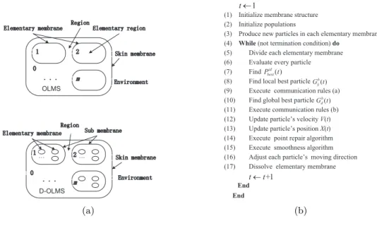
In mMPSO, a dynamic membrane structure (specifically, OLMS alternates with D-OLMS shown in Fig. 3(a)) is introduced to arrange a population of particles, each of which is a feasible path for a mobile robot, and specify various rules, such as membrane division, transformation and communication-like rules, and membrane dissolution. The dimension of each particle is variable in the process of evolution. The point repair algorithm described above is used to change infeasible paths into feasible ones. The repair process may increase the dimensions of each particle. The smoothness algorithm presented in this section is applied to remove the redundant nodes of a path and the process may decrease the dimensions of each particle. In
addition, a moving direction adjustment technique is presented to accelerate the algorithm convergence. The pseudocode algorithm of mMPSO is shown in Fig. 3(b), where each step is described in detail as follows:
(OHPHQWDU\PHPEUDQH 5HJLRQ(OHPHQWDU\UHJLRQ (QYLURQPHQW 6NLQPHPEUDQH P (OHPHQWDU\PHPEUDQH 6XEPHPEUDQH 6NLQPHPEUDQH (QYLURQPHQW 5HJLRQ P OLMS D-OLMS (a)
(1) Initialize membrane structure
(2) Initialize populations
(3) Produce new particles in each elementary membrane
(4) While(not termination condition)do
(5) Divide each elementary membrane
(6) Evaluate every particle
(7) Find
(8) Find local best particle
(9) Execute communication rules (a)
(10) Find global best particle
(11) Execute communication rules (b)
(12) Update particle’s velocityV(t) (13) Update particle’s position X(t)
(14) Execute point repair algorithm
(15) Execute smoothness algorithm
(16) Adjust each particle’smoving direction
(17) Dissolve elementary membrane
End End +1 t¬t Begin: 1 t¬ ( ) b d G t ( ) id best P t ( ) b ij G t (b)
Figure 3: Membrane structures and the pseudocode algorithm for mMPSO
Step 1: An OLMS [[ ]1, . . . ,[ ]m]0 composed of a skin membrane denoted by 0 and m+ 1
regions inside the skin membrane is constructed. The way in which the parameter m is chosen will be discussed in Section 4.
Step 2: A particle swarmX with m particles in a D-dimensional search space is randomly generated and each particle is put inside an elementary membrane in OLMS, whereDrepresents the number of nodes in a feasible path;X ={x1, x2, . . . , xm}, wherexi is an arbitrary individual
inX and denotes a feasible path, xi = (xi1, xi2, . . . , xiD).
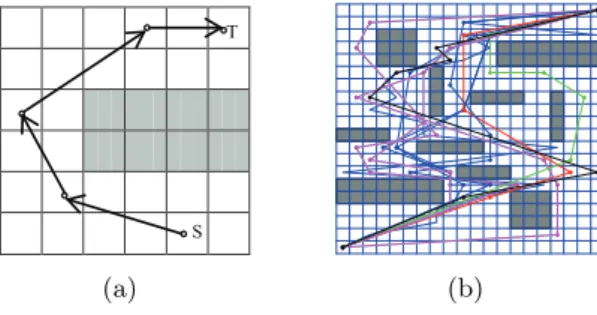
Step 3: In this step, a moving direction adjustment technique is introduced to produce n
particles inside each elementary membrane. To be specific, we modify the velocity of the particle inside each elementary membrane to generate a new particle by using (6) and (7),
V(g+ 1) =ρ1·Vr(g) +ρ2·Vf(g) (6)
X(g+ 1) =X(g) +V(g+ 1) (7)
whereρ1 andρ2are the inertia weighting factors and usually are set to larger values for exploring
the global solutions;Vr(g) is the randomly produced velocity of thegth particle (at the beginning
for each elementary membrane,g=0);Vf(g) is the adjusted velocity of thegth particle by using
the idea of tightening fishing line and the moving directions of each node in thegth particle is shown in Fig. 4(a); V(g+ 1) is the velocity of the (g+ 1)th particle; X(g) and X(g+ 1) are positions of the gth and (g+ 1)th particles. Inspired by the idea of tightening fishing line, we consider a feasible path as a fishing line and tighten the line from the target node, thus, each node except for the target one in the path will show a moving direction toward the next node (the target node is the first one). The moving directions of all the nodes in the path construct the velocityVf(g). This step is repeated for ntimes to producennew particles for each elementary
membrane and used together with the point repair algorithm and smoothness algorithm. The dimensions of new particles may be greater than or less than D. Thus, the swarm will have
m×nparticles in total. Fig. 4(b) shows an example that one particle with 20 dimensions (the thick line) inside a certain elementary membrane produces 10 particles with 6–10 dimensions (the thin line). Compared to the random approach, the production of the new particles can remove redundant nodes of a path and has better adaptability in hostile environment, especially in the circuitous route environment.
S T
(a) (b)
Figure 4: An example of the generation of new particles and direction of each dimension of the individual
Step 4: The maximal number of iterations is used as the termination condition.
Step 5: This step first classifies the n particles inside the ith elementary membrane into
ki clusters according to the dimension of each particle and then divides the ith elementary
membrane into ki membranes, each of which contains the particles with the same dimension,
i= 1,2, . . . , m. Thus, OLMS becomes D-OLMS.
Step 6: Each particle is evaluated by using (1) and assigned a fitness value.
Step 7: Find Pid
best(t), which is the best solution of each particle in its history with respect
to the fitness values.
Step 8: Find the locally best solution Gbij(t) in the jth elementary membrane inside theith membrane,i= 1,2, . . . , m, j= 1,2. . . , ki, in terms of fitness values.
Step 9: Perform communication rules (a), which first send all the locally best solutionsGbij(t) (j = 1,2. . . , ki) out into the ith submembrane, i= 1,2, . . . , m, and further send out into the
skin membrane.
Step 10: Find the globally best solutionGbd(t) by comparingGbij(t) with the same dimension
d,d∈ {1,2, . . . , D},i= 1,2, . . . , m, j = 1,2. . . , ki.
Step 11: Perform communication rules (b), which send Gbd(t) back into the elementary membrane containingd-dimension particles across certain submembrane.
Step 12: Update the velocities of thed-dimension particles using (8).
Vid(t+ 1) =δ1· ρ·Vid(t) +c1·r1· Pbestid (t)−Xid(t) +c2·r2· Gbij(t)−Xid(t) +c3·r3· Gdb(t)−Xid(t) +δ2·Vidf(t) (8) whereVid(t) andVid(t+ 1) are the velocities of the particle at generationtandt+1, respectively;
Pbestid (t) is the best solution of the particle at generation t; Xid(t) is the position the particle
at generation t; Gbij(t) is the locally best solution with the same dimension d at generation
t; Gbd(t) is the globally best solution with the same dimension d at generation t; Vidf(t) is the adjusted velocity of the particle at generation t; δ1 and δ2 are proportion coefficients; ρ is
an inertia weighting factor; r1, r2 and r3 represent the functions that generate independently
random numbers, which are uniformly distributed between 0 and 1;c1,c2andc3 are acceleration
coefficients.
Step 13: Update the positions of the d-dimension particles using (9).
whereXid(t) andXid(t+ 1) are the positions of the particle at generationtandt+1, respectively;
Vid(t+ 1) is the velocity of the particle at generation t+ 1.
Step 14: Execute point repair algorithm for each particle.
Step 15: Execute smoothness algorithm for each particle.
Step 16: Adjust the moving direction of each particle by using the moving direction adjust-ment technique.
Step 17: This step dissolves all the elementary membranes and releases their particles into their corresponding submembranes. Thus, D-OLMS becomes the original OLMS.
4
Experimental Results
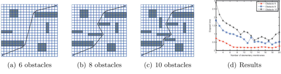
The mMPSO performance is tested by using MR3P. We first discuss how to set the number
m of elementary membranes in OLMS by using 20 ×20 grid model environment with 6, 8 and 10 obstacles, respectively. Then, 16×16 grid model environment with 9 static obstacles are applied to compare mMPSO with its counterpart vPSO and GA [15]. Subsequently, the complex environments, 32×32 and 64×64 grid model environments with 20 static obstacles, are applied to further test the mMPSO performance. In these experiments, one dynamic obstacle representing a moving obstacle or a dangerous source occurring suddenly is employed to analyze the mMPSO behavior.
(a) 6 obstacles (b) 8 obstacles (c) 10 obstacles
2 4 6 8 10 12 14 16 18 20 0 0.5 1 1.5 2 2.5 3
Number of elementary membranes
E la p se d t im e Obstacle 6 Obstacle 8 Obstacle 10 (d) Results
Figure 5: The near shortest paths in three environments (20×20 grid with obstacles 6, 8 and 10, respectively) and experiment results
4.1 Parameter Setting
In this subsection, we use 20×20 grid model environment with three kinds of obstacles shown in Fig. 5 to discuss how to choosem. Fig. 5(a)-(c) have 6, 8, 10 static obstacles (shaded areas), respectively. In the following experiments, the population size is set to 100; In (8),
c1 = c2 =c3 = Gsize/Vmax, where Gsize = 0.08 is the size of a grid and Vmax is the maximal
distance allowing a node to move in a step; the proportion coefficientsδ1= 0.65,δ2= 0.35; ρis
defined as a variable, which varies from 0.246 to 0.157 along the logarithm function log10(y). In (6), ρ1 and ρ2 are set to random values between 0.4 and 0.6. In (3), α= 0.6,β= 0.4. In (4), λ
is set to the robot radius.
In what follows,mvaries from 2 to 20 by an increment of 2, thus, we first generatemparticles inStep 2 and inStep 3 for the first m−1 elementary membranes, we produceround(100/m) particles and 100−(m−1)∗round(100/m) particles for the mth elementary membrane, where
round(.) is a function for rounding its element towards nearest integer. In the experiments, if a given near-optimal solution is reached, mMPSO stops. Because the optimal solution to MR3P is usually unknown, we set Kd = 1, Ks = Kf = 0 in (1) and independently perform mMPSO
S T r1=0,r2=1 r1=1,r2=0 (a) ! (b) S T r1=0,r2=1 r1=1,r2=0 (c)
Figure 6: Experimental results of mMPSO in the environments 16×16 grids,Os= 9 andOd= 1.
S T r1=0,r2=1 r1=1,r2=0 (a) 32×32 S r1=0,r2=1 r1=1,r2=0 (b) 32×32 S T (c) 32×32 S T r1=0,r2=1 r1=1,r2=0 (d) 64×64
Figure 7: Experimental results of mMPSO in the environments 32×32, 64×64 grids,Os= 20
and Od= 1.
set to 2000, in order to find the near-optimal solution. Fig. 5(a)-(c) show the near shortest paths of the model environment with different obstacles, 6, 8 and 10, respectively. The mMPSO performance for each of the 19 cases is evaluated by using the mean of the elapsed time in 30 independent runs. The experimental results are shown in Fig. 5(d), where the elapsed time for three environments first decreases and then increases as the value of m goes up. These experimental results indicate thatm could be 13 by considering the three environments.
4.2 MR3P Experimental Results
To investigate the mMPSO performance, this subsection uses three grid models, 16×16, 32×32 and 64×64, to carry out the experiments and considers five environments: 16×16 with 9 static obstacles (Os = 9), 16×16 with Os = 9 and one dynamic obstacle (Od = 1),
32×32 withOs= 20, 32×32 with Os = 20 and Od = 1, 64×64 with Os= 20. The place for
the possible occurrence of the dynamic obstacle is set to the near center, which is very likely to block the feasible paths. The model with 16×16 grids is applied to compare mMPSO with its counterpart PSO (vPSO) and GA in [15]. The models with 32×32 and 64×64 grids are used to further discuss the mMPSO performance in different complex environments. The setting of the parameters in mMPSO except for Kd, Ks, Kf is the same as in Subsection 4.1. m=13.
The termination condition is designated as the maximal number 2000 of iterations. All the experiments are run on the PC with CPU 1.7GHz, 512MB RAM, and the software platform MATLAB7.4 and Windows XP OS.
We first use the model with 16×16 grids to compare mMPSO with vPSO (when m = 1, mMPSO becomes vPSO) and GA in [15]. We consider three cases forKd, Ks, Kf as follows:
(1) Case 1: Kd= 1, Ks=Kf = 0, γ1= 1, γ2 = 0;
(2) Case 2: Kd= 0.6, Ks=Kf = 0.2, γ1 = 0, γ2= 1;
(3) Case 3: Kd= 0.8, Ks+Kf = 0.2, γ1+γ2= 1.
Method NoO NoNO NoI Fv Gn St
GA[36] 9 78 13 24.68 16 1.68
vPSO 83 108 0 24.95 65 2.97
mMPSO 94 239 0 24.26 27 0.84
Table 1: Comparisons of three methods in the environment(Fig. 6 (a))
Method NoO NoNO NoI Fv Gn St
GA[36] 32 68 0 24.71 12 0.69
vPSO 81 103 0 28.56 73 3.12
mMPSO 92 235 0 27.43 34 0.97
Table 2: Comparisons of three methods in the environment(Fig. 6 (c))
best path in Case 1 considering only one objective, path length, and the red line is the best result in Case 2 by trading-off safety and smoothness. Fig. 6(b) illustrates 8 near optimal paths (8 colors) through balancing the path length, safety and smoothness. The paths in Fig. 6(c) are obtained by considering one dynamic obstacle and the blue line is the best path in Case 1 considering only one objective, path length, and the red line is the best result in Case 2 by trading-off safety and smoothness.
To draw a comparison with GA in [15] and vPSO, let Kd=1 and the experiment is
exe-cuted for 100 independent runs. Tables 1 and 2 show the experimental results of GA, vPSO and mMPSO for the environments with static obstacles and the environments with static and dynamic obstacles. In Tables 1-3 , NoO, NoNO, NoI, Fv, Gn, St represents the number of optimal solutions, the number of near optimal solutions, the number of infeasible solutions and the fitness value in 100 trials, the average generations for finding the optimal solution and the mean of the elapsed time(s) in each trial, respectively.
As it can be clearly seen from Table 1 and Fig. 6, mMPSO finds much more optimal paths and near optimal paths, while it spends smaller computing time than GA. There are some infeasible solutions in GA, while there is not any infeasible solution in vPSO and mMPSO because the point repair algorithm have repaired the infeasible path. On the other hand, vPSO also finds more optimal paths and near optimal solutions than GA, but the elapsed time is far larger than GA. mMPSO is better than vPSO with respect to optimal and near optimal solutions and the elapsed time, which indicates the advantage of the combination of a membrane system with PSO. Table 2 shows similar conclusions to those in Table 1.
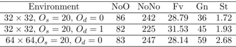
To further analyze the mMPSO performance in more complex environments, more experi-ments are conducted in the environexperi-ments with 32×32 and 64×64 grids containing 20 or 21 obstacles, as shown in Fig. 7 (a-d). The environment with 32×32 grids and 20 static obstacles
Environment NoO NoNo Fv Gn St
32×32,Os= 20,Od= 0 86 242 28.79 36 1.72
32×32,Os= 20,Od= 1 82 225 31.53 45 1.93
64×64,Os= 20,Od= 0 83 247 28.14 59 2.68
are shown in Fig. 7 (a). Fig. 7(b)-(c) show the environment with 20 static obstacles and one dynamic obstacle. In Fig. 7 (c), the three objectives, path length, smoothness and safety, are considered. The parameters of mMPSO are the same as above except for the population size 150 andm= 15. All the tests are executed for 100 independent runs. Table 3 shows the results. It can be seen from Tables 1-3 that the optimal solutions of mMPSO drop from 94 to 83, the elapsed time rises from 0.84 to 2.68 and the average generations vary from 27 to 59 as the number of cells increases from 16×16 to 64×64 and the static obstacles go up from 9 to 20. The elapsed time and average generations increase a little with the dynamic obstacle. To sum up, as the number of cells increases in accordance with 4n(n= 1,2,3. . .) values and the static obstacles double, the increase in the elapsed time is quite small, as opposed to an exponential growth in cells number. mMPSO maintains good search capability to find the optimal solution in both static and dynamic environments, which indicates mMPSO has good adaptability to MR3P under complex environments.
5
Conclusions
This paper discusses a feasible combination of membrane systems and PSO to solve MR3P. The outstanding novelty is to justify the introduced dynamic membrane structure, which proves to be suitable for solving MR3P with variable dimensions. mMPSO uses the alternation of OLMS and D-OLMS to integrate a PSO with variable dimensions, point repair algorithm, smoothness algorithm and moving direction adjustment. A large number of experiments are carried out on several MR3P with various environments and the results show that mMPSO can achieve much better solutions than its counterparts PSO and GA, as reported in the literature.
This paper considers only the planar (two dimensions) environments. Following this work, we aim to further investigate how to extend mMPSO to three dimensional spaces, how to use mMPSO to solve more difficult path planning problems (mobile robots follow the tracks of moving targets in a hostile environments), how to combine mMPSO with numerical P systems to control mobile robots and how to apply the idea of variable dimension PSO to solve other engineering problems.
Acknowledgment
The work of XW, GZ, JZ and HR was supported by the National Natural Science Foundation of China (61170016, 61373047), the Program for New Century Excellent Talents in University (NCET-11-0715) and SWJTU supported project (SWJTU12CX008). The work of FI and RL was supported by a grant of the Romanian National Authority for Scientific Research, CNCS-UEFISCDI, project number PN-II-ID-PCE- 2011-3-0688.
References
[1] P˘aun, Gh.; Rozenberg, G.; Salomaa, A. eds,(2010); The Oxford handbook of membrane computing, Oxford University Press.
[2] P˘aun, Gh. (2007); Tracing some open problems in membrane computing,Rom J Inform Sci Tech, ISSN 1453-8245, 10(4): 303–314.
[3] Zhang, G.X.; Pan, L.Q. (2010); A survey of membrane computing as a new branch of natural computing, Chinese J Computer, ISSN 0254-4164, 33(2): 208–214.
[4] Nishida T.Y. (2004); An application of P system: a new algorithm for NP-complete opti-mization problems. Proc 8th WMCSCI, 109–112.
[5] Zhang, G.X.; Gheorghe, M.; Pan, L.Q.; P´erez-Jim´enez, M.J. (2014); Evolutionary membrane computing: a comprehensive survey and new results, Inform Sci (accepted).
[6] Huang, L.; He, X.; Wang, N.; Xie, Y. (2007); P systems based multi-objective optimization algorithm, Prog Nat Sci, ISSN 1002–0071, 17(4): 458-465.
[7] Zhang, G.X.; Gheorghe, M.; Li, Y. (2012); A membrane algorithm with quantum-inspired subalgorithms and its application to image processing, Nat Comput, ISSN 1567-7818, 11(3): 701–717.
[8] Zhang, G.X.; Cheng, J.X; Gheorghe, M. (2014); Dynamic behavior analysis of membrane-inspired evolutionary algorithms, Int J Comput Commun Control, ISSN 1841-9836, 9(2): 227–242.
[9] Kennedy, J.; Eberhart, R. (1995); Particle swarm optimization,Proc ICNN, 4: 1942–1948. [10] Zhang, G.X.; Zhou, F.; Huang, X.L; Cheng, J.X; Gheorghe, M; Ipate, F.; Lefticaru, R.
(2012); A novel membrane algorithm based on particle swarm optimization for solving broad-casting problems, J Univers Comput Sci, ISSN 0948-6968 18(13): 1821–1841.
[11] Xiao, J.; Huang, Y.; Cheng, Z; He, J; Niu, Y. (2014); A hybrid membrane evolutionary algorithm for solving constrained optimization problems, Optik, ISSN 0030-4026, 125(2): 897–902.
[12] Lozano-P´erez, T.; Wesley, M.A. (1979); An algorithm for planning collision-free paths among polyhedral obstacles, Commun ACM, ISSN 0001-0782, 22(10): 560–570.
[13] Gao, H.; Cao, J. (2012); Membrane quantum particle swarm optimisation for cognitive radio spectrum allocation, Int J Comput Appl Tech, ISSN 0952-8091, 43(4): 359–365. [14] Hwang, Y.K.; Ahuja, N. (1992); Gross motion planning - A survey, ACM Comp Surv, 24:
219-291.
[15] Tuncer, A.; Yildirim, M. (2012); Dynamic path planning of mobile robots with improved genetic algorithm, Comput Electr Eng, ISSN 0045-7906, 38: 1564–1572.
[16] Garcia, M.A.; Montiel, O. (2009); Path planning for autonomous mobile robot navigation with ant colony optimization and fuzzy cost function evaluation, Appl Soft Comput, ISSN 1568-4946, 9(3): 1102–1110.
[17] Qidan, Z.; Yang, Y.J.; Xing, Z.Y. (2006); Robot path planning based on artificial potential field approach with simulated annealing, Proc ISDA, 622–627.
[18] Zhang, Y.; Gong, D.W. (2013); Robot path planning in uncertain environment using multi-objective particle swarm optimization, Neurocomputing, ISSN 0925-2312, 103: 172–185. [19] Masehian, E.; Sedighizadeh, D. (2007); Classic and heuristic approaches in robot motion
planning - A chronological review, Proc. WASET, 101–106.
[20] Xu, W.F.; Li, C.; Liang, B. (2008); The cartesian path planning of free-floating space robot using particle swarm optimization, Int J Adv Rob Syst, ISSN 1729-8806, 5: 301–310.
[21] Gong, D.W.; Zhang, J.H. (2011); Multi-objective particle swarm optimization for robot path planning in environment with danger sources, J Comput, 6(8): 1554–1561.