Vision-based Obstacle Avoidance for Small UAVs

Worcester Polytechnic Institute

Digital WPI

Major Qualifying Projects (All Years)

Major Qualifying Projects

April 2015

Vision-based Obstacle Avoidance for Small UAVs

Cy M. Ketchum

Worcester Polytechnic Institute

Kevin Philip Hancock

Worcester Polytechnic Institute

Sam Louis Friedman

Worcester Polytechnic Institute

Follow this and additional works at:

https://digitalcommons.wpi.edu/mqp-all

This Unrestricted is brought to you for free and open access by the Major Qualifying Projects at Digital WPI. It has been accepted for inclusion in Major Qualifying Projects (All Years) by an authorized administrator of Digital WPI. For more information, please [email protected].

Repository Citation

Ketchum, C. M., Hancock, K. P., & Friedman, S. L. (2015).Vision-based Obstacle Avoidance for Small UAVs. Retrieved from

Abstract

Autonomous obstacle avoidance is a fundamental desirable feature of all unmanned aerial vehicles (UAVs). Due to severe payload weight restrictions, small UAVs are limited in the number and type of sensors that can be carried on-board for detecting and avoiding the environment. This project describes an obstacle avoidance system based on two lightweight off-the-shelf cameras, and a small Raspberry Pi microcontroller. The system was designed to receive telemetry and sensor data from the UAV’s basic autopilot and to return command guidance for to avoid obstacles in the desired path. To implement this system, algorithms for object tracking and depth mapping using monocular and stereo camera vision were adapted. Workbench tests and flight tests on the IRIS quadrotor UAV were performed.

”Certain materials are included under the fair use exemption of the U.S. Copyright Law and have been prepared according to the fair use guidelines and are restricted from further use.”

Acknowledgments

We would like to thank the following individuals for their help and support throughout the entirety of this project.

Project Advisor: Professor Raghvendra Cowlagi Computing Support: Raffaele Potami

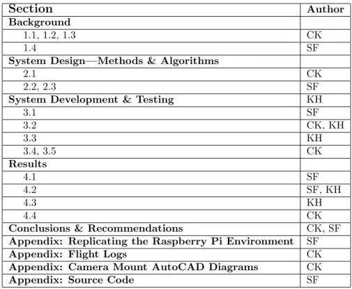
Table of Authorship

Section

Background

1.1, 1.2, 1.3 CK

1.4 SF

System Design—Methods & Algorithms

2.1 CK

2.2, 2.3 SF

System Development & Testing KH

3.1 SF 3.2 CK, KH 3.3 KH 3.4, 3.5 CK Results 4.1 SF 4.2 SF, KH 4.3 KH 4.4 CK

Conclusions & Recommendations CK, SF

Appendix: Replicating the Raspberry Pi Environment SF

Appendix: Flight Logs CK

Appendix: Camera Mount AutoCAD Diagrams CK

Contents

1 Background 6

1.1 UAV Development . . . 6

1.2 Current Uses of UAVs . . . 6

1.3 Research Frontiers . . . 7

1.4 Obstacle Detection . . . 8

2 System Design—Methods & Algorithms 8 2.1 Sensor Selection . . . 8

2.2 Computer Vision . . . 9

2.3 Camera Calibration . . . 10

3 System Development & Testing 11 3.1 Bench Testing . . . 11 3.2 Quadcopter Selection . . . 13 3.2.1 IRIS . . . 13 3.2.2 AscTec Pelican . . . 14 3.2.3 Spiri . . . 14 3.3 Quadcopter Simulation . . . 14 3.3.1 Gazebo . . . 15 3.3.2 Spiri Simulator . . . 15

3.3.3 In-Simulation Depth Mapping . . . 15

3.4 Quadcopter Setup . . . 16

3.4.1 Radio Receiver Calibration . . . 16

3.4.2 Electronic Speed Controller calibration . . . 17

3.4.3 Radio Telemetry Calibration . . . 17

3.4.4 Accelerometer Calibration . . . 18

3.4.5 Compass Calibration . . . 19

3.5 Quadcopter Payload . . . 19

3.5.1 Preparation of the Cameras . . . 19

3.5.2 Design and Construction of the Payload . . . 20

4 Results 23 4.1 Depth Mapping . . . 23

4.2 Object Detection . . . 24

4.3 Real-time Object Detection . . . 26

4.4 Flight Testing . . . 27

5 Conclusions & Recommendations 27 6 Appendix: Replicating the Raspberry Pi Environment 31 6.1 Installing the Operating System . . . 31

6.2 Installing Required Packages . . . 31

7 Appendix: Flight Logs 32 8 Appendix: Camera Mount AutoCAD Diagrams 34 9 Appendix: Source Code 35 9.1 Camera Calibration . . . 35

1

Background

This section provides background knowledge on the subject of unmanned aerial vehicles. This includes a brief history of UAV development, examples of the current use of UAVs, and current research frontiers in the field. Additionally, this section provides information on the topics of obstacle detection and obstacle avoidance, which are fundamental to this project.

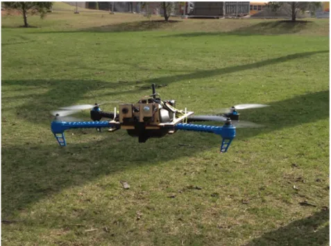
Figure 1: Our fully-assembled depth-mapping system in flight.

1.1

UAV Development

Throughout history, UAV technology has undergone incredible advancements. Experimentation with UAVs began soon after the first manned flight, however practical results were not achieved until the First World War [1]. Early UAVs were little more than primitive missiles and few were actually used in combat. Around the time of the Vietnam War, the use of UAVs for surveillance, intelligence, and reconnaissance became more common [1]. In the present day, UAVs have a large number of applications and have achieved widespread use in many fields. Due to advancements in UAV technology, unmanned vehicles can perform dangerous tasks at a lower cost and without risking human life. The continued development of UAV technology holds incredible potential for the future.

1.2

Current Uses of UAVs

Unmanned aerial vehicles have an extensive variety of applications and can be used to perform tasks that would be difficult or impossible for humans. One area that UAVs are commonly associated with is the military. The history of unmanned aircraft used for combat purposes extends back well over fifty years. Early systems were primitive, but advances in technology have greatly increased the capabilities and potential of modern craft [2]. Micro UAVs are often used for observation purposes in hostile areas, as their portability and low cost makes them invaluable assets in the field. Larger UAVs can carry powerful and accurate sensors to gather information without placing a pilot in danger [3]. Military applications of UAVs are constantly developing and decreasing costs are allowing their usage to proliferate [2].

The use of UAVs is not limited to military purposes. For example, forestry has benefited greatly from the use of unmanned vehicles. UAVs have been equipped with infrared sensors in conjunction with computer vision to detect and localize forest fires. This system provides a more mobile and perceptive platform than ground-based robots [5]. UAVs have been used in conjunction with LIDAR sensors in order to take inventory of forests, including determination of tree heights and locations. This provides

Figure 2: Military UAV [4]

forest managers with more data and enables them to make more informed administrative decisions [6]. Additionally, UAVs have been used to support search and rescue missions. A UAV equipped with a camera may help expedite the search for victims [7]. In addition to their commercial and professional applications, UAVs are also frequently used recreationally by hobbyists to record videos from the air and show off with aerobatic stunts.

Figure 3: UAV spotting an early stage forest fire [8]

1.3

Research Frontiers

UAV technology has advanced greatly since its inception and has come to new research frontiers. A future advancement for UAVs is increased usage in the field of civil aviation. However, there are many barriers that must be worked around before this can become possible. These barriers include regulation barriers, such as unmanned airspace and certifications, as well as technology barriers, such as communication, data acquisition, and perception [9].

UAVs involve complex systems and there are many variables that must be considered during devel-opment and operation. Path planning for UAVs is constantly evolving, including algorithms for obstacle detection and avoidance[10]. These are concepts that are central to this project.

1.4

Obstacle Detection

In order to reduce dependence of a UAV on human operators, autonomous control is required. In navigating a desired path, an autonomous UAV must take into account static and dynamic obstacles such as buildings, terrain, other vehicles, and people. The successful avoidance of such obstacles is dependent on accurate obstacle detection logic [11]. There are a number of sensing schemes that may provide the needed environment data, the most commonly implemented of which are computer vision, LIDAR [12] and sonar [13] schemes. Ground-based robots have developed far enough to use suites of combined sensor types [14], though their relatively constant proximity to the ground enables the use of novel approaches not available to air-based platforms [12] [15]. Instead, most research in UAV obstacle detection in recent years has taken advantage of the relatively low cost and light payload weight of vision-based systems [16]. These systems are also flexible in their design: different numbers of sensors may be used, with different obstacle detection algorithms in each situation. Most commonly, either one or two cameras are used to provide environment data. In the case of a single camera, features such as edges or corners are identified and tracked from one sensor frame to the next in a process known as optical flow. In dual-camera implementations, the disparity of pixels between the left and right sensors is used to compute a depth mapping [17] [18]. It has also been shown that a combination of these methods is possible, using cameras of different framerate to perform both stereo correspondence and feature tracking [19]. These computer vision approaches are made easier by the availability of software packages built for the implementation of computer vision algorithms. One such package, OpenCV, was selected for use in this project due to the completeness of its feature-set and its implementation in both C++ and Python [20].

2

System Design—Methods & Algorithms

2.1

Sensor Selection

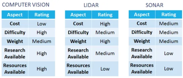
At the inception of the project, it was necessary to decide what system would be used for obstacle detection. There were three main options available; computer vision, LIDAR, and sonar. In order to make a selection, the feasibility of each option was examined.

Computer vision is a fairly low-cost system, as it can be implemented for only the cost of usable cameras. The difficulty to implement usable computer vision algorithms is quite high, however there is a great deal of research on the subject available and there are many free resources with which to begin work. LIDAR was an option that is commonly used with obstacle detection. By using a mounted laser, range and intensity measurements are analyzed in order to determine the existence of an obstacle [21]. One major limitation to the use of a LIDAR system for this project was the price, as many of these systems can cost hundreds or even thousands of dollars. Additionally, the payload required for a LIDAR system is comparatively heavy. It was important to minimize the payload size for this project as the IRIS quadcopter has a limited carrying capacity. The final system, sonar, is also commonly used for obstacle detection. The basic function of a sonar detection system operates by emitting a sound wave and measuring the time required for it to be reflected back. The distance can then be calculated by dividing the speed of sound by this time. Sonar fell in the middle range of the examined systems, as the price point was generally between computer vision and LIDAR. However, there were comparatively few resources and research available for designing a sonar system.

It was determined that computer vision would be used for this project due to the low cost and high amount of resources available. While the expected difficulty was high, it was expected that the large availability of research and resources would help to offset any problems encountered.

Figure 4: Comparison of potential sensors

2.2

Computer Vision

To implement the stereo depth mapping system, the team used a Python-accessible implementation of the OpenCV computer vision library. This gave access to complex vision algorithms such as stereo correspondence without needing to implement these algorithms in Python. The OpenCV library is written in C however, and this fact may be a source of latency and inefficiency in the system.

The core of the depth-mapping system is the generation of a disparity map. A disparity map uses two images—one from each of a stereo camera pair—to generate a mapping of movement of the pixels in an image between cameras.

Figure 5: Geometric diagram of disparity determination.

In the above image, the camera sensors are at points O and O’. The object being mapped is at point X. Each camera is separated by a baseline distance, B. The cameras have inherent optical properties, including a focal length. The focal length of the cameras may be used to determine the location of the cameras’ ”image plane”, or the plane on which the image appears to have been taken. Longer focal lengths ”zoom” the image more, while very short focal lengths may produce extremely large fields-of-view. Point X is projected to each camera’s image plane to form points x and x’.

The disparity of each pixel from image x to x’ is simplyx−x0. By constructing similar triangles, the depth, Z, of point X can be written as

Z = B·f

x−x0

In this equation,Bis a value in meters, andf andx,x0 are values in pixels. By calculating the disparity of each pixel in the image and then applying the operation defined above, the result is a depth map of the

input images. The depth map pixels have the same relative values as the disparity map pixels, but their values have been modified so as to correspond to distance measurements. A professionally photographed stereo image pair was used to test this implementation.

Figure 6: Proof-of-concept of disparity and depth mapping.

The accuracy of the result may be tweaked by adjusting the two parameters of OpenCV’s stereo correspondence matcher, ”StereoBM”. StereoBM uses the ”Block-Match” algorithm, and takes as argu-ments the number of disparities as well as the block size. In the algorithm, the number of disparities is an integer value (divisible by 16 so as to correspond to the square search location) that defines the maximum levels of disparity allowed in the depth map. A value of 0 corresponds to an unlimited number of levels. The block size is an integer value corresponding to the size of the blocks into which the block-match algorithm breaks the image to search for correspondences. In the above image, combinations of these parameters and their results are shown.

2.3

Camera Calibration

Through the disassembly of the camera sensors as well as their inherently low quality as consumer hardware, the cameras contributed a large amount of error—and thus noise—to the depth map. This error can be offset if the distortion of each camera is known: the captured images are simply un-distorted through application of an appropriate transformation. In OpenCV, this can be done via the calibrateCamera method and its supporting functions.

Section 7 includes the source code used to calibrate the cameras. In this process, OpenCV polls a camera looking for a checkerboard pattern. When such a pattern is found, OpenCV records the position of the corners of the checkerboard. After a number (10-20) of images are taken, OpenCV can compare the expected position of the checkerboard corners to their position in each image. This allows the program to generate a summary of the distortion found in the camera’s images. OpenCV returns a ”camera matrix”, containing the camera’s focal length as well as its distortion coefficients. Further, the program returns a ”region of interest” describing the portion of the image deemed to be of acceptably low-distortion.

Figure 7: An example image from the calibration process.

Again likely due to the inexpensive nature of the cameras, the error found in the calibration process was higher than expected. RMS error of the camera matrices was often 0.5 or higher. Additionally, each camera’s region-of-interest was often wildly different. Since a full anti-distortion algorithm would crop each image to its region-of-interest, this presents a problem: the depth-mapping algorithm requires images of the same dimensions. For these reasons, camera calibration was limited to gaining more accurate measures of the cameras’ focal length. In the future, more accurate cameras would likely reduce these problems.

3

System Development & Testing

3.1

Bench Testing

For the bench-testing and development system, Ubuntu Linux 12.04.5 was used due to its support from both the OpenCV computer vision library as well as the Spiri Gazebo simulator. The code was developed in Python, due to the team’s existing familiarity with the language. Further, Python would be easily portable to the on-board Raspberry Pi computer of the UAV payload. In setting up the worksta-tion, a number of development packages and tools were required. A list of these requirements is below, followed by a recounting of the procedure for the setup of these tools on both the workbench and the Raspberry Pi.

Development Stack:

1. Python 2.x

2. GCC, CMake & related build-tools 3. OpenCV 2.4.9.0

4. ROS Hydro 5. Gazebo 6. Spiri Simulator

Ubuntu 12.04.5 includes Python, but it was necessary to install C-code building tools before using the Python implementation of OpenCV. This can be done simply from the package manager:

Now the OpenCV library can be built from source. The source is easily downloadable from OpenCV’s repository: http://sourceforge.net/projects/opencvlibrary/.

The downloaded file will contain a directory named ”opencv”. In this directory a working directory called ”release” is created:

>$ cd ~/opencv >$ mkdir release >$ cd release

Then, configure and build:

>$ cmake -D CMAKE_BUILD_TYPE=RELEASE -D CMAKE_INSTALL_PREFIX=/usr/local ..

And then, to make and install the library:

>$ make

>$ sudo make install

These same steps can be followed on the Raspberry Pi to configure the environment there.

ROS Hydro is required to support Spiri Simulator, as it is the backbone for the Gazebo simulation environment. It can easily be installed from the package manager, but we first need to add the ROS repositories to our package sources:

>$ sudo sh -c ’echo "deb

http://packages.ros.org/ros/ubuntu precise main" > /etc/apt/sources.list.d/ros-latest.list’ >$ wget https://raw. githubusercontent.com/ros/rosdistro/ master/ros.key -O - |

sudo aptkey add

-Now, install:

>$ sudo apt-get update >$ sudo apt-get install ros-hydro-desktop-full

And now set-up ROS for use:

>$ sudo rosdep init >$ rosdep update

>$ echo "source /opt/ros/ hydro/setup.bash" >> ~/.bashrc

>$ source ~/.bashrc >$ sudo apt-get install python-rosinstall

Finally, the Spiri simulator can be installed, which will be used for testing vision code. Spiri’s developers have provided an easy-to-use installation script.

>$ wget https://raw.github.com/ Pleiades-Spiri/Spiri_Public/ Simulator-alpha-1.1/installation.sh >$ wget https://raw.github.com/ Pleiades-Spiri/Spiri_Public/ Simulator-alpha-1.1/ installation_simulator.sh >$ chmod +x installation.sh installation_simulator.sh >$ ./installation.sh

And then simply reload the terminal and run the installer:

>$ bash --login

>$ ./installation_simulator.sh

3.2

Quadcopter Selection

To determine a suitable quadcopter to use for this project, a variety of products from various manu-facturers were researched. The products that were examined are detailed in this section.

3.2.1 IRIS

Figure 8: The IRIS quadcoptor [22]

The IRIS quadcopter was made available by the project adviser at the start of the project. The IRIS, a product of 3DRobotics, is equipped with a Pixhawk autopilot system, which led to the decision to use an on-board processing platform with a Raspberry Pi as the two are can communicate via MAVlink. MAVlink is a communication standard used to send commands and information to and from UAV autopilot boards. Developers can implement the MAVlink standard in various ways; we identified one implementation—MAVProxy—for use on Raspberry Pi. The IRIS was used throughout the entirety of this project, however other potential options were explored. While researching other possible flight platforms, the IRIS was prepared for flight tests by performing calibrations and constructing a mount for the on-board system.

3.2.2 AscTec Pelican

Figure 9: The AscTec Pelican [23]

The AscTec Pelican was the first option that was explored for a flight platform due to the variety of available components, such as a platform that could accommodate several different sensors. At this point in the project, the use of LIDAR was being considered, which made the Pelican a viable option due to the different options for LIDAR sensors that were available. The team contacted the AscTec manufacturers about the packages available for the Pelican, such as the different camera mounting systems. A quote was obtained for the Pelican and several cameras and sensors. However, the high price point and the fact that the company is based in Germany (necessitating importation) made placing an order for the Pelican a long, difficult process. As such, the project proceeded using the IRIS quadcopter.

3.2.3 Spiri

Figure 10: The SPIRI quadcopter [24]

Another quadcopter that that was examined during the research phase was Spiri. The Spiri quad-copter is a Kickstarter project that caught the interest of the team due to the built-in stereo cameras, the bottom-mounted camera (for altitude determination), and the simulation software that was available. An order was placed for Spiri and the simulation was examined during the meantime. However, the expected delivery date changed unexpectedly to late March, after the project was expected to conclude. This necessitated that the project move forward using the IRIS.

3.3

Quadcopter Simulation

In order to eliminate the need to reload software onto a physical test platform and to bring said platform to an outside location to perform the test, the team decided to utilize pre-existing simulation packages for ROS (Robotic Operating System) and Gazebo. The pre-existing packages were used for the simulation of both the control software and physical hardware.

3.3.1 Gazebo

Gazebo is robotic simulation software designed to work with platforms which utilize ROS: the Robot Operating System, designed to enable programmatic description and modeling of robotic sys-tems. Gazebo provides an environment in which nearly all real world sensors and control systems can be implemented and emulated to provide meaningful simulation results. With Gazebo one can test and rapidly make changes without having to constantly having to update a physical system and bring this system to a testing location. The ability to both accurately simulate the stereo cameras and eliminate the need to bring the system to an outside location for testing after each modification made Gazebo worth looking into.

Though Gazebo is a promising platform for the simulation and test of our depth-mapping algorithms, it proved too complicated a system to allow for the full implementation of the testing model in the avail-able time. The team was avail-able to test disparity mapping and control concepts using availavail-able packages, but elected to focus on the development of the depth-mapping system instead of creating a higher-fidelity Gazebo model of the system.

3.3.2 Spiri Simulator

The Spiri Simulator was used to simulate the stereo cameras required for depth mapping and object detection. After downloading and installing the Spiri package, the simulation software Gazebo could be opened by opening two terminals and launching Spiri within an empty world and keyboard teleoperation:

>$ roslaunch spiri_description spiri_empty_world.launch

>$ roslaunch spiri_teleop keyboard_teleop.launch

3.3.3 In-Simulation Depth Mapping

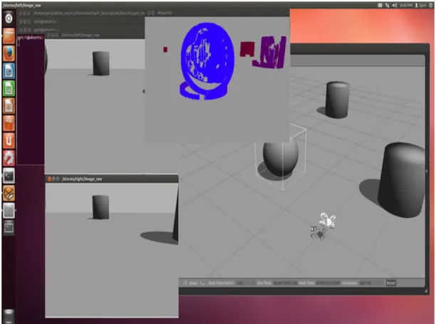
By launching Gazebo with an empty world and keyboard controls for Spiri, it was possible to simulate a basic quadrotor with a simplified control scheme. In order to begin the simulation of the front facing cameras and built in depth mapping it was necessary to first initialize the left and right cameras, then run the depth mapping algorithm, and then view the output of the algorithm:

>$ rosrun image_view image_view image:=/stereo/left/image_raw >$ rosrun image_view image_view image:=/stereo/right/image_raw

>$ ROS_NAMESPACE=stereo rosrun stereo_image_proc stereo_image_proc _approximate_sync:=True _queue_size: >$ rosrun image_view stereo_view stereo:=/stereo image:=image_rect_color _approximate_sync:=True _queue

Figure 11: Disparity mapping in Gazebo

Figure 5 is an example of one of the team’s tests on the stereo camera imaging and depth mapping in gazebo. In the figure, a simulation of Spiri is being run in an enviornment with multiple objects at various distances. Displayed are Spiri’s two front facing cameras and the correspoding disparity map of the objects produced by the two cameraa.

3.4

Quadcopter Setup

The IRIS was designated to be the flight platform for a camera payload. Mission Planner software was installed on a ground station laptop to collect and process telemetry data and perform some calibration procedures.

After performing a preliminary test flight with the IRIS, it was determined that the calibration was not correct. The calibration procedure involved several steps, including calibration of the radio receiver, electronic speed controllers, radio telemetry, accelerometers, and compass. Throughout the calibration process, flight tests were conducted on the Higgins House Lawn with the permission of WPI police. These test flights helped determine whether the calibration procedures were working and whether the telemetry was operational. Flight tests were mostly performed in the manual (ALT) mode of flight, although some tests used the self-stabilizing (STB) mode. A log of the flight tests is included in the appendix.

3.4.1 Radio Receiver Calibration

The radio receiver calibration was performed in accordance with the procedure detailed in the Iris Advanced Manual [25].

1. Connect the battery to IRIS and connect IRIS to the ground station computer. Turn on the RC transmitter.

2. Open Mission Planner and change the communication port to the option that displays PX4. Set the Baud rate to 115200 and press “Connect”.

3. Go to the “Initial Setup” menu. Open the subsection “Mandatory Hardware” and then “Radio Calibration”. Press the “Calibrate Radio” button.

4. On the RC transmitter, rotate the sticks in large circles so the input limits can be recorded. Calibration of the radio receiver improved the responsiveness of IRIS during flight.

3.4.2 Electronic Speed Controller calibration

After one of the flight tests, two of the motors on the quadcopter stopped performing properly. The motors would not engage unless the throttle was set to its maximum. In order to rectify this problem, the electronic speed controllers (ESCs) were calibrated using instructions from the Arducopter wiki [26].

1. Remove the propellers and any USB connectors from IRIS

2. Turn on the RC transmitter and set the throttle all the way forward

3. Connect the battery to IRIS. The autopilot should light up with red, blue, and yellow. Disconnect and reconnect the battery.

4. Press and hold the safety button on IRIS until it displays solid red. IRIS is now in ESC calibration mode.

5. Wait for IRIS to emit a series of beeps. This indicates that the maximum throttle has been recorded.

6. On the RC transmitter, pull the throttle down to its minimum position. IRIS should emit a long tone to indicate that calibration is complete.

7. Test the motors by raising and lowering the throttle. Set the throttle to minimum and disconnect the battery.

Subsequent to the ESC calibration, the motors once again performed at full capacity.

3.4.3 Radio Telemetry Calibration

IRIS is able to collect telemetry data via two 3DR radios; one is installed inside IRIS and acts as an air module, and the other is connected to the ground station by micro USB to act as the ground module. There was initially a problem where the two radios were not communicating. After contacting 3DRobotics customer support, the team determined that the problem was that the two network IDs of the radios were different. Radio calibration was performed to correct this problem.

Figure 12: 3DR radio [27] 1. Open Mission Planner on the ground station

2. Connect the ground station radio to the ground station

3. Click on “Initial Setup”→“Optional Hardware”→“3DR Radio” 4. Click on “Load Settings”

5. Make a note of the value of the Net ID 6. Disconnect the ground station radio 7. Open the shell of the IRIS

8. Unplug the air module from the PIXHAWK autopilot (it does not need to be physically removed from IRIS)

9. Connect the air module to the ground station via micro USB 10. Click on “Initial Setup”→“Optional Hardware”→“3DR Radio” 11. Click on “Load Settings”

12. Check the value of the Net ID. If it is different from the Net ID of the ground module, change the value so that the two Net IDs are the same.

13. Click “Save Settings”

14. Disconnect the air module from the ground station.

In order to check that the connection is working properly, connect the battery to IRIS and the ground station radio to the ground station. In Mission Planner, select the ground station COM port, set the baud rate to 57600, and click “Connect”. Mission Planner will display whether the connection is successful.

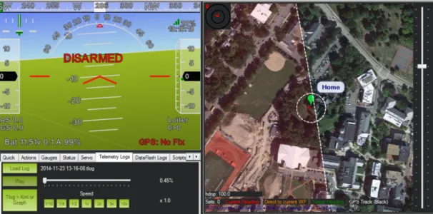
Once telemetry was functioning properly, we used it during our flight tests to record data about IRIS’s flight. This data included flight speeds, flight heading, and other information about IRIS’s performance.

Figure 13: Example telemetry log recorded by IRIS

3.4.4 Accelerometer Calibration

The accelerometer was calibrated in an effort to reduce the listing of the quadcopter during flights, which was a problem that had been identified during flight testing. In order to accomplish this, the team followed the accelerometer calibration steps on the arducopter wiki [28].

1. Connect the battery to IRIS and connect IRIS to the ground station computer. Turn on the RC transmitter.

2. Open Mission Planner and change the communication port to the option that displays PX4. Set the Baud rate to 115200 and press “Connect”.

3. Click on “Initial Setup”→“Mandatory Hardware”→“Accelerometer Calibration” 4. Click on “Calibrate Accel”

5. Follow the instructions given by Mission Planner

Once the accelerometer was calibrated, the performance of IRIS improved dramatically. The listing was almost entirely eliminated, and maintaining control of IRIS during flight became much easier.

3.4.5 Compass Calibration

In an effort to improve IRIS’s performance during IRIS’s self-stabilizing flight mode (STB), the compass was calibrated by following the steps in the arducopter wiki [28].

1. Connect the battery to IRIS and connect IRIS to the ground station computer. Turn on the RC transmitter.

2. Open Mission Planner and change the communication port to the option that displays PX4. Set the Baud rate to 115200 and press “Connect”.

3. Click on “Initial Setup”→“Mandatory Hardware”→“Compass” 4. Check the “Enable” and “Auto Dec” boxes and click “Live Calibration” 5. Select the Pixhawk autopilot

6. Follow the Mission Planner prompt and hold the copter in the air, slowly rotating it about every axis

7. When calibration is complete, a window will pop up with the results

After calibration, IRIS’s STB mode was moderately more balanced, but it was determined that the manual mode was easier and more comfortable to fly with.

3.5

Quadcopter Payload

In order to ensure that the on-board processor and cameras could be carried by IRIS, it was necessary to construct a mount. For this payload the Raspberry Pi, the webcams, and a power source had to be secured. The mounting system began as a conceptual design that was later refined and constructed before being tested in the field.

3.5.1 Preparation of the Cameras

The cameras used for this project were the Microsoft Lifecam HD 3000 model. These cameras were specifically designed to be webcams, but were re-purposed to work for the purposes this project. First, the camera sensor was extracted by disassembling the webcam casing. This sensor was then spliced with a USB connector by soldering the wires together. This allowed the cameras to be plugged into the Raspberry Pi’s USB ports and be easily integrated into the payload.

Figure 14: Disassembled webcam.

3.5.2 Design and Construction of the Payload

The first conceptual design for the payload involved using the GoPro camera mount on the front of IRIS. The plan was to attach a platform to this mount where the cameras could be secured. Additionally, the Raspberry Pi was to be secured to the top of IRIS using wire, which would be achievable by going through the vent slits on the top of the shell. However, when the processor was moved on-board, the design was altered and refined further.

Figure 15: Conceptual payload mount.

In order to acquire usable images, it was important to minimize the motion of the cameras. To ensure this, the team designed a mount that would allow the cameras to be securely fastened to IRIS. In this

mount, a layer of foam and wood was placed on each side of the camera sensor and secured with a bolt. This was done in order to minimize any vibrations that may occur during flight.

Figure 16: Securing the camera sensor.

In order to implement an on-board processor, the IRIS payload required a power source. A battery pack for the Raspberry Pi was constructed by using a step-down converter and four AA batteries. This DIY battery pack was made for about ten dollars, the price of the converter. The battery pack connects to the Raspberry Pi’s general purpose input/output pins and can provide up to ten hours of battery life. Due to the limited flight time of the IRIS (roughly fifteen minutes per battery), this was more than sufficient for the purposes of this project.

Figure 17: Battery pack for the Raspberry Pi

mounted vertically to take front-view images. By placing a bolt through the setup and attaching a nut to the back, the motion of the cameras was minimized. Additionally, the slot allowed for the position of the cameras to be adjusted if necessary.

Figure 18: Camera mount with slotted base.

In order to secure this camera payload as well as an on-board power source for the Raspberry Pi, a body-mounted frame was designed. This design featured a slotted platform at the front of IRIS to hold the camera payload and an additional platform on the back for the battery pack to sit on. This measure, along with the inherent inertial navigation system in the Pixhawk autopilot, ensured that the weight distribution of the payload did not interfere with flight. This frame was designed to sit on top of the arms of IRIS and was secured by braces placed underneath.

Figure 19: Body-mounted frame for camera payload.

All of the models for the parts required for the mount were designed with SolidWorks. By importing the SolidWorks files to AutoCAD, it was possible to manufacture them using a laser cutter. The material used was quarter-inch thick birch plywood.

Figure 20: Dimensioned (inches) AutoCAD drawing of body-mounted frame.

Once all of the parts were cut, the payload could be constructed. The battery pack was secured to the back platform with tape, while the camera payload was inserted into the slotted front platform. The Raspberry Pi was top mounted, and any stray wires for the camera and power source connections were secured to the shell.

Figure 21: Fully assembled payload.

4

Results

4.1

Depth Mapping

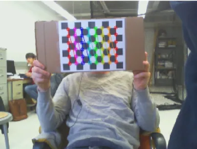
Once the workbench tests on the stereo imaging system began, extent of the camera sensors’ noise and distortion became apparent. The results of one of the team’s earliest tests, shown below, illustrate the high noise in both the disparity and the depth maps. In this test, the top-left image is the disparity map and the top-right image is the depth map. Below these maps, the source images from the left and right camera can be viewed. In the last row of images, the source frames are subtly transformed according to the distortion found in the camera calibration algorithm and converted to grayscale as required by the stereo correspondence algorithm.

Figure 22: The depth-mapping rig in testing.

As is shown in the above figure, the stereo imaging is correctly identifying the checkerboard object in center view of the frame, but inconsistently calculates its disparity and corresponding depth. While this test was of only a static frame on a work bench, the results provided enough accuracy that the team was confident that with the correct filtering method the calculated depth map would allow for quasi-object detection.

4.2

Object Detection

In order to obtain meaningful object detection, it was necessary to utilize some form of data refine-ment. The final method chosen was to take a certain region and to then average all of the depths within said region to calculate a final measurement of “mean depth”. The mean depth was calculated both over the entire image as well as in a central region. The image in figure 19 shows the smaller region’s location within the yellow box in both the left and right image. This approach was designed to emphasize the field-of-view most likely to contain problematic objects: straight-ahead of the IRIS.

After determining the method of filtering the team then designed a test procedure to determine the accuracy of the depth-mapping algorithm. Using the checkerboard pattern from the camera calibration procedure as the test object, the stereo camera rig was placed one meter away from the test object. The test object was moved closer to the camera rig by five inches after the collection of ten data points at each distance. The results of this test are shown in the figure below.

Figure 23: Results of depth-mapping at a distance from 1m to 0.2m.

As is shown in figure 20, the calculated results for both the full and central area approximate the trend shown by the Actual Distance series, but a bias has placed them at a negative intercept. The full area depth has better adherence to the trend at high distances. By offsetting the full area depth series we can view its correlation to the Actual Distance line, as shown in the transparent red series in the figure below.

Figure 24: The previous graph with bias accounted for in the transparent red series.

Here we see that the system is producing data that is fairly accurate, and extremely repeatable. The most accurate region seems to be the region of distances from 1 meter to 0.5 meters. To further examine the accuracy in this region, a second test was conducted with more data points from 1 meter to 0.5

meters.

Figure 25: A second test in the most promising distance region of 1m to 0.5m.

As evidenced by the above figure, the system is very accurate in the region of 1 meter to 0.5 meters. The trend largely adheres to the Actual Distance, differing above and below the expected trend at different points in the series. This is likely due to our use of only a simple linear bias; in reality, camera parameters and distortion are causing a more complex bias to occur in our data. Correcting this bias could be done via a calibration procedure for the depth map; at each test distance the system could compare expected and actual distance and generate a bias. By using a range of biases as distance changes, a more accurate result can be achieved.

4.3

Real-time Object Detection

After calibration of the camera for static images, the next test to be run was for real-time object detection. The test ran the static depth-mapping algorithm in a continual loop, then wrote ”Object Detected” to the console if mean depth below a chosen distance was calculated for the central or full area regions. The figure below is the example of one such test, where an object is moved in front of the system to trigger the ”center object detected”.

Figure 26: Real-time test of object detection algorithm

In the figure above, the algorithm is displaying the calculated mean depth values for both the full area (the left column) and the central area (the right column).

The stereo imaging rig performed well on the test bench, with frame rates nearing one frame per second and with very few false positives. After the positive results achieved in the lab, the code was

migrated to the Raspberry Pi in anticipation for real-world testing. Slight modifications had to be made due to the inability to read the console while the IRIS was in flight. During flight-test, the Raspberry Pi wrote test data to a log file with time stamps, and recorded each image frame to a separate data directory so that the source images and output data could be compared after flight to determine if the system was correctly identifying objects in the flight path.

4.4

Flight Testing

Once the camera payload was attached to the IRIS, flight tests were conducted on the Higgins House lawn. The Raspberry Pi ran the same configuration as for the bench test; taking depth map readings periodically and saving images to the SD card. The quadcopter was able to lift off with no observed problems, and handled normally. This served as an indication that the payload was balanced properly and the Pixhawk’s inertial navigation system was able to deal with the applied load. The quadcopter was flown around the lawn and near trees to determine if the obstacle detection was functioning properly. After the flight, the photos and data taken were examined. However, the data that was recorded indicated that there was a problem with the camera offset as compared to the lab tests. It is possible that the cameras reacted differently to the natural lighting and thus the offset required for the cameras was different. Additionally, many of the flight photos showed signs of overexposure, which could have affected the collected data.

Figure 27: Sample photos taken during flight testing.

5

Conclusions & Recommendations

Over the course of this project, the team evaluated different sensor options before choosing to work with computer vision in order to develop an obstacle detection system. The team was able to implement a DIY stereo depth mapping system capable of mounting on a small UAV. Through camera calibration and bench testing, a stereo imaging algorithm was developed. The bench testing results showed that the depth algorithm was highly precise, but more tuning and bias-correction must be performed in order to increase the accuracy. The Raspberry Pi was identified as a capable on-board processor, and a payload and mount were designed and built to allow the IRIS quadcopter to perform flight tests with the stereo imaging system. The results showed that more specialized hardware is required for implementation in the field. Finally, the team created recommendations on how to move forward with this project in the future.

There are three main recommendations to make for a future group working with this project. The first recommendation is the implementation of a control loop. With a functional control loop, upon detection of an obstacle a command could be sent to halt the motion of the quadcopter. The MAVProxy API system that represents dimensional motion with variables is a simple method for sending control commands. With this system, it should not be overly difficult to implement a control loop. This would additionally bring the system closer to functioning autonomously.

The second recommendation is to optimize the code of this project for real-time speed. Currently, the vision code is written in Python. However, OpenCV runs on C. Since stereo correspondence is a highly expensive algorithm, the maximum processing speed of the system as-is results in one frame of

depth-processing per second. The transliteration of this code to C would likely result in faster depth mapping. With this and possibly the addition of a faster on-board processor, real-time optimization should be achievable.

The third recommendation is in regards to the camera calibration and parameters. During the camera calibration for this project it was apparent that the Microsoft webcams had high error in their optical properties. The error and inconsistency between these cameras is a potential cause for the bias and offsets experienced during the camera testing. It is recommended to research and acquire higher-quality stereo vision cameras as they will likely exhibit more consistencies and improved results.

Continued study will allow the results achieved over the course of this project to be further refined and expanded upon. By using specialized stereo cameras and exporting the code to C, it is likely that many of the equipment problems can be mitigated. The implementation of a control loop would bring the project closer to the eventual goal of an on-board autonomous obstacle avoidance system.

References

[1] J. D. Blom,Unmanned Aerial Systems: A Historical Perspective, vol. 45. Combat Studies Institute Press, 2010.

[2] K. L. Cook, “The silent force multiplier: the history and role of uavs in warfare,” in Aerospace Conference, 2007 IEEE, pp. 1–7, IEEE, 2007.

[3] A. C. Watts, V. G. Ambrosia, and E. A. Hinkley, “Unmanned aircraft systems in remote sensing and scientific research: Classification and considerations of use,” Remote Sensing, vol. 4, no. 6, pp. 1671–1692, 2012.

[4] S. Frink, “General atomics aeronautical systems releases upgrade for predator b/mq-9 uav.” web, sep 2012.

[5] L. Merino, F. Caballero, J.-d. Dios, and A. Ollero, “Cooperative fire detection using unmanned aerial vehicles,” in Robotics and Automation, 2005. ICRA 2005. Proceedings of the 2005 IEEE International Conference on, pp. 1884–1889, IEEE, 2005.

[6] G. Grenzd¨orffer, A. Engel, and B. Teichert, “The photogrammetric potential of low-cost uavs in forestry and agriculture,”The International Archives of the Photogrammetry, Remote Sensing and Spatial Information Sciences, vol. 31, no. B3, pp. 1207–1214, 2008.

[7] S. Waharte and N. Trigoni, “Supporting search and rescue operations with uavs,” in Emerging Security Technologies (EST), 2010 International Conference on, pp. 142–147, IEEE, 2010.

[8] T. Frey, “We have officially entered the drone era,” mar 2013.

[9] T. Warchocki, Autonomy research for civil aviation : toward a new era of flight. Washington, D.C: The National Academies Press, 2014.

[10] H. Duan and P. Li, “Uav path planning,” inBio-inspired Computation in Unmanned Aerial Vehicles, pp. 99–142, Springer, 2014.

[11] M. Becker, C. M. Dantas, and W. P. Macedo, “Obstacle avoidance procedure for mobile robots,” in

ABCM Symposium series in Mechatronics, vol. 2, pp. 250–257, 2006.

[12] J. Han, D. Kim, M. Lee, and M. Sunwoo, “Enhanced road boundary and obstacle detection using a downward-looking lidar sensor,” Vehicular Technology, IEEE Transactions on, vol. 61, no. 3, pp. 971–985, 2012.

[13] H. P. Moravec and A. Elfes, “High resolution maps from wide angle sonar,” in Robotics and Au-tomation. Proceedings. 1985 IEEE International Conference on, vol. 2, pp. 116–121, IEEE, 1985. [14] R. Manduchi, A. Castano, A. Talukder, and L. Matthies, “Obstacle detection and terrain

classifi-cation for autonomous off-road navigation,”Autonomous robots, vol. 18, no. 1, pp. 81–102, 2005. [15] I. Ulrich and I. Nourbakhsh, “Appearance-based obstacle detection with monocular color vision,”

inAAAI/IAAI, pp. 866–871, 2000.

[16] Y. Watanabe, A. J. Calise, and E. N. Johnson, “Vision-based obstacle avoidance for uavs,” inAIAA Guidance, Navigation and Control Conference and Exhibit, pp. 20–23, 2007.

[17] R. Jain, R. Kasturi, and B. G. Schunck,Machine Vision. McGraw-Hill New York, 1995.

[18] Y. Morvan, “Acquisition, compression and rendering of depth and texture for multi-view video,” 2009.

[19] S. Shen, Y. Mulgaonkar, N. Michael, and V. Kumar, “Vision-based state estimation for autonomous rotorcraft mavs in complex environments,” inRobotics and Automation (ICRA), 2013 IEEE Inter-national Conference on, pp. 1758–1764, IEEE, 2013.

[20] G. Bradski and A. Kaehler,Learning OpenCV: Computer vision with the OpenCV library. ” O’Reilly Media, Inc.”, 2008.

[21] J. Hancock, M. Hebert, and C. Thorpe, “Laser intensity-based obstacle detection,” in Intelli-gent Robots and Systems, 1998. Proceedings., 1998 IEEE/RSJ International Conference on, vol. 3, pp. 1541–1546, IEEE, 1998.

[22] A. Copter, “Iris - the ready to fly uav quadcopter.” Web, 2015. [23] A. Technologies, “Asctec pelican.” Web.

[24] RobotShop, “Spiri 1.0 quadcopter development platform.” Web, 2015. [25] Arduino,Iris Advanced Manual. Arducopter, 2014.

[26] Arducopter,ESC Calibration. 3DRobotics, 2014. [27] 3DRobotics, “3dr radio set.” web, 2015.

6

Appendix: Replicating the Raspberry Pi Environment

The following instructions may be used to fully replicate our Raspberry Pi production environment, including all required packages and programs.

Requirements:

1. A Raspberry Pi microcomputer. We used the model B+, but at the time of writing the latest model is the Raspberry Pi 2. These instructions aim to be independent of hardware version. 2. A micro-SD card having at least 16GB capacity.

3. A micro-SD to SD card adapter, to enable use on a desktop computer.

6.1

Installing the Operating System

We performed all development and testing under the Raspbian Linux distribution. This distribution of Linux can be easily downloaded and installed following the provided guide for your operating system,

found at the Raspberry Pi Foundation website: http://www.raspberrypi.org/documentation/installation/installing-images/README.md

6.2

Installing Required Packages

Below are enumerated the major packages and programs used in the project. Specific commands will follow to install these packages and any required dependencies.

1. Python: the programming language in which our code is built. 2. OpenCV: an image-processing library.

3. Numpy: a scientific utility library for Python used by OpenCV. 4. guvcview: a utility used to test USB cameras.

5. MAVproxy: the Python program used to communciate with Pixhawk.

First we will update our system to be sure that all existing packages and available packages are up to date:

>$ sudo apt-get update >$ sudo apt-get upgrade

Now we can begin installing packages:

>$ sudo apt-get install libopencv-dev python-opencv

This will install the latest version of OpenCV and all requried dependencies including Python and Numpy. Next we will install guvcview so that we can test our cameras to ensure they work as expected:

>$ sudo apt-get install guvcview

Now we can install the required packages for MAVproxy to enable communication with the Pixhawk autopilot.

>$ sudo apt-get install screen python-wxgtk2.8 python-matplotlib python-pip python-numpy

Any already installed packages and dependencies will be ignored. Finally we must configure the Rasp-berry Pi to disable the login prompt on its serial port: this allows us to send and receive data via the pinout without needing to authenticate - something the Pixhawk cannot do.

>$ sudo nano /etc/inittab

This will open a text editor. Use the arrow keys to scroll to the bottom of the file, and type a # character at the beginning of the last line so that it appears as:

#TO:23:respawn:/sbin/getty -L ttyAMA0 115200 vt100

Then press Ctrl+X, then Y to confirm exit, and then the Enter key to save the file. Now reboot with the following command:

>$ sudo reboot now

Your Raspberry Pi is now configured to run our control code and communicate with a Pixhawk board.

7

Appendix: Flight Logs

1. Tuesday, 10/14/14 Flight area: A J Knight Field Flight time: 2:30pm Weather conditions: clear Flight testing began on A J Knight Field due to lack of flying permissions for the football and soccer fields. Flight testing encountered some difficulties due to the small flying space. This and the proximity to the highway make the A J Knight Field a less than ideal flying location.

The quadcopter listed heavily to one side during the flights.

2. Saturday, 10/25/14 Flight area: Higgins House Lawn Flight time: 1pm Weather conditions: clear, windy

Radio calibration was performed on the quadcopter prior to flight, as according to the instructions listed on the arducopter site

Subsequent to the calibration, the control was better but there were still difficulties with the wind and listing of the quadcopter.

3. Sunday, 10/26/14 Flight area: Higgins House Lawn Flight time: 1pm Weather Conditions: clear, windy

Due to the wind, control was fairly difficult to maintain. One propeller sustained damage due to an unexpected landing.

4. Friday, 11/7/14 Flight area: Higgins House Lawn Flight time: 4pm Weather Conditions: clear, very windy

After the first flight test was conducted, the wind was judged to be too strong to continue flying. Controlling the quadcopter was very difficult under the weather conditions.

Radio telemetry was not functional during this flight. After calling the 3DR help service, the net IDs of the two radios not matching was identified as a potential problem.

5. Saturday, 11/8/14 Flight area: Higgins House Lawn Flight time: 4pm Weather Conditions: clear Flight testing during this day was successful. The quadcopter handled well and did not encounter problems during flight.

Radio telemetry was not functional during this flight. Subsequent to the flight, there was an attempt to change the net ID of the radio inside the quadcopter so that it matched the net ID of the ground station radio. However, there was an error upon connection.

6. Sunday, 11/9/14 Flight area: Higgins House Lawn Flight time: 3pm Weather conditions: clear Flight testing during this day encountered problems. After one of the flight attempts, the two right-most propellers stopped spinning under idling conditions. Further testing in the lab concluded that the propellers would only spin when max throttle was induced. The problem was later identified to be a miscalibration of the ESCs that cause the motors to spin. Upon calibration, following the instructions in the arducopter wiki, the problem was fixed.

Radio telemetry was not functional during this flight. Subsequent to the flight, the net ID of the radio inside the quadcopter was fixed to match the ground station radio. This was accomplished by first opening up the shell of the quadcopter, unplugging the radio from the Pixhawk inside the quadcopter, and then connecting to the radio with a micro USB. When both are connected at once, they share a com port which does not allow the radio to connect with the ground station properly. After the net id was changed, the two radios successfully connected.

7. Friday, 11/14/14 Flight area: Higgins House Lawn Flight time: 4pm Weather conditions: windy Flight testing during this day encountered difficulties. The quadcopter listed heavily to one side which made control difficult to maintain.

Flight telemetry was successfully operational during this day and a telemetry log was obtained. 8. Saturday, 11/15/14 Flight area: Higgins House Lawn Flight time: 3pm Weather conditions: windy

Flight testing during this day was delayed due to a heavy presence of people around Higgins House due to a wedding/sporting event.

Subsequently, accelerometer calibration was performed on the quadcopter using the steps detailed on the arducopter wiki.

9. Sunday, 11/16/14 Flight area: Higgins House Lawn Flight Time: 2pm Weather conditions: light wind

Flight testing during this day was a success. The accelerometer calibration worked well and all but eliminated listing during flight.

Telemetry logs were recorded for this flight.

10. Wednesday, 11/19/14 Flight area: Higgins House Lawn Flight time: 12pm Weather conditions: windy

Flight testing was successful in spite of the wind. Group members took turns flying the copter. The copter calibration seemed functional, however loiter mode did not work properly. One propeller was damaged during an abrupt landing.

Flight telemetry was not active during this test flight.

11. Friday, 11/21/14 Flight area: Higgins House Lawn Flight time: 4pm Weather conditions: windy During this test, the loiter function on the quadcopter was tested in order to see whether the copter could hover on its own. Prior to flight, compass calibration was performed using the procedure detailed here: http://copter.ardupilot.com/wiki/initial-setup/configuring-hardware/

Loiter mode seemed to be functioning properly, however it was difficult to determine due to the wind. Additionally, the return to launch function was determined to be functioning properly. Flight telemetry was active during this flight.

12. Saturday, 11/22/14 Flight area : Higgins House Lawn Flight time: 1pm Weather conditions: windy This flight was cut short due to low charge on the batteries. It was indeterminable whether loiter mode was working. Will try again tomorrow.

13. Sunday, 11/23/14 Flight area: Higgins House Lawn Flight time: 1pm Weather conditions: clear, minimal wind

During this flight, we tried the loiter function on the quadcopter. Loiter was functional, however it was determined that the ALT mode is the best suited for flight tests due to allowing the most control.

8

Appendix: Camera Mount AutoCAD Diagrams

Figure 28: Dimensioned (inches) AutoCAD drawing of front of camera mount.

Figure 29: Dimensioned (inches) AutoCAD drawing of back of camera mount.

9

Appendix: Source Code

9.1

Camera Calibration

This file defines a function for calibrating a camera using checkerboard corner-finding. When the function is called, Python will poll the chosen camera for frames and search these frames for a checker-board pattern of the desired dimensions. Once this pattern is found, Python will wait for a chosen number of successful pattern recognitions. It will then use the OpenCV method ”calibrateCamera” to return a calibration matrix from the input checkerboard frames.

import numpy a s np

import cv2

def c a l i b r a t e c a m e r a ( cam , name , g r i d w i d t h , g r i d h e i g h t ) :

# t e r m i n a t i o n c r i t e r i a

c r i t e r i a = ( cv2 . TERM CRITERIA EPS + cv2 . TERM CRITERIA MAX ITER, 3 0 , 0 . 0 0 1 )

# p r e p a r e o b j e c t p o i n t s , l i k e ( 0 , 0 , 0 ) , ( 1 , 0 , 0 ) , ( 2 , 0 , 0 ) . . . . , ( 6 , 5 , 0 )

o b j p = np . z e r o s ( ( g r i d h e i g h t∗g r i d w i d t h , 3 ) , np . f l o a t 3 2 )

o b j p [ : , : 2 ] = np . mgrid [ 0 : g r i d h e i g h t , 0 : g r i d w i d t h ] . T . r e s h a p e (−1 ,2)

# Arrays t o s t o r e o b j e c t p o i n t s and image p o i n t s from a l l t h e i m a g e s .

o b j p o i n t s = [ ] # 3 d p o i n t i n r e a l w o r l d s p a c e

i m g p o i n t s = [ ] # 2 d p o i n t s i n image p l a n e .

n u m s u c c e s s = 0

cv2 . namedWindow ( ’Raw Image ’ ) cv2 . namedWindow ( ’ Corner Find ’ )

while n u m s u c c e s s < 2 0 :

f r a m e r e t , img = cam . r e a d ( )

g r a y = cv2 . c v t C o l o r ( img , cv2 .COLOR BGR2GRAY) cv2 . imshow ( ’Raw Image ’ , g r a y )

# Find t h e c h e s s b o a r d c o r n e r s

r e t , c o r n e r s = cv2 . f i n d C h e s s b o a r d C o r n e r s ( gray , ( g r i d h e i g h t , g r i d w i d t h ) , None )

print r e t

# I f found , add o b j e c t p o i n t s , image p o i n t s ( a f t e r r e f i n i n g them )

i f r e t == True : o b j p o i n t s . append ( o b j p ) cv2 . c o r n e r S u b P i x ( gray , c o r n e r s , ( 1 1 , 1 1 ) , (−1 ,−1 ) , c r i t e r i a ) i m g p o i n t s . append ( c o r n e r s ) # Draw and d i s p l a y t h e c o r n e r s cv2 . d r a w C h e s s b o a r d C o r n e r s ( img , ( g r i d h e i g h t , g r i d w i d t h ) , c o r n e r s , r e t ) cv2 . imshow ( ’ Corner Find ’ , img )

n u m s u c c e s s += 1 print ”Found c o r n e r s : s u c c e s s e s = ” + s t r( n u m s u c c e s s ) cv2 . waitKey ( 1 0 0 ) #c v 2 . waitKey ( 1 ) print ”Got r e q u i r e d c a l i b r a t i o n i m a g e s : p e r f o r m i n g c a l i b r a t i o n . . . ” r e t , mtx , d i s t , r v e c s , t v e c s = \ cv2 . c a l i b r a t e C a m e r a ( o b j p o i n t s , i m g p o i n t s , g r a y . s h a p e [ : :−1 ] , None , None ) print ” C a l i b r a t i o n m a t r i c e s c r e a t e d . E r r o r = ” + s t r( r e t ) cv2 . d e s t r o y A l l W i n d o w s ( ) # g e t new camera m a t r i x f r a m e r e t , img = cam . r e a d ( ) h , w = img . s h a p e [ : 2 ]

newcameramtx , r o i=cv2 . getOptimalNewCameraMatrix ( mtx , d i s t , ( w, h ) , 1 , ( w, h ) ) print( ” W r i t i n g mtx” ) print(s t r( mtx ) ) np . s a v e ( ’ mtx ’+name+ ’ . npy ’ , mtx ) print( ” W r i t i n g d i s t ” ) print(s t r( d i s t ) ) np . s a v e ( ’ d i s t ’+name+ ’ . npy ’ , d i s t ) print( ” W r i t i n g newcameramtx ” ) print(s t r( newcameramtx ) )

np . s a v e ( ’ newcameramtx ’+name+ ’ . npy ’ , newcameramtx )

print( ” W r i t i n g r o i ” ) print(s t r( r o i ) ) r o i f i l e = open( ’ r o i ’+name , ’w ’ ) r o i f i l e . w r i t e (s t r( r o i ) ) r o i f i l e . c l o s e ( ) return

9.2

Depth Mapping

The file ”generate depth map.py” defines the functions needed to poll the stereo camera rig for frames and generate disparity maps on these frames. The file ”get test data.py” defines a test procedure using the depth mapping code in ”generate depth map.py”.

from math import s q r t

import cv2 import t i m e import numpy a s np from m a t p l o t l i b import p y p l o t a s p l t import m a t p l o t l i b . cm a s cm def rms ( a r r a y ) : n = np . s i z e ( a r r a y ) return s q r t ( ( 1 / n )∗np .sum( a r r a y∗ ∗2 ) ) def t e s t d e p t h ( a r r a y ) : i f np . mean ( a r r a y ) < 1 : return True e l s e: return F a l s e

def make depth map ( d o p l o t , b i a s , n u m d i s p a r i t i e s , b l o c k s i z e , s t a r t t i m e , now ) : p l t . c l o s e ( ” F i g u r e 0 ” )

# C r e a t e camera o b j e c t s , g e t i m a g e s

capL = cv2 . VideoCapture ( 0 )

i f not capL . isOp ened ( ) : print( ” L e f t Camera F a i l e d ” ) r e t L , o r i g f r a m e L = capL . r e a d ( )

capL . r e l e a s e ( )

capR = cv2 . VideoCapture ( 1 )

i f not capR . isOp ene d ( ) : print( ” R i g h t Camera F a i l e d ” ) retR , o r i g f r a m e R = capR . r e a d ( )

# Depth mapping p a r a m e t e r s b a s e l i n e = 0 . 0 5 3 9 7 5 # m e t e r s f o c a l = 445 # p i x e l s b f P r o d u c t = b a s e l i n e∗f o c a l # F i r s t v a l u e i s number o f d i s p a r i t i e s ( d i v i s i b l e by 1 6 ) # s e c o n d v a l u e i s b l o c k s i z e ( odd no . ) p a r a m e t e r s = ( n u m d i s p a r i t i e s , b l o c k s i z e )

# Load camera c a l i b r a t i o n s − uncomment i f u n d i s t o r t i n g i m a g e s ## p r i n t ( ” C a l i b r a t i n g l e f t camera . . . ” )

## mtxL = np . l o a d ( ’ mtxL . npy ’ ) ## d i s t L = np . l o a d ( ’ d i s t L . npy ’ )

## newcameramtxL = np . l o a d ( ’ newcameramtxL . npy ’ ) ## r o i L = f i l e ( ’ r o i L ’ ) . r e a d ( ) ## r o i L = r o i L . r e p l a c e ( ’ ( ’ , ’ ’ ) . r e p l a c e ( ’ ) ’ , ’ ’ ) . r e p l a c e ( ’ , ’ , ’ ’ ) ## r o i L = t u p l e ( [ i n t ( s ) f o r s i n r o i L . s p l i t ( ) i f s . i s d i g i t ( ) ] ) ## p r i n t ( ” C a l i b r a t i n g r i g h t camera . . . ” ) ## mtxR = np . l o a d ( ’ mtxR . npy ’ ) ## d i s t R = np . l o a d ( ’ d i s t R . npy ’ )

## newcameramtxR = np . l o a d ( ’ newcameramtxR . npy ’ ) ## roiR = f i l e ( ’ roiR ’ ) . r e a d ( ) ## roiR = roiR . r e p l a c e ( ’ ( ’ , ’ ’ ) . r e p l a c e ( ’ ) ’ , ’ ’ ) . r e p l a c e ( ’ , ’ , ’ ’ ) ## roiR = t u p l e ( [ i n t ( s ) f o r s i n roiR . s p l i t ( ) i f s . i s d i g i t ( ) ] ) #uncomment i f u s i n g s t a t i c t e s t i m a g e s : ## o r i g f r a m e L = c v 2 . imread ( ” . / t o w e r l e f t . j p e g ” ) ## o r i g f r a m e R = c v 2 . imread ( ” . / t o w e r r i g h t . j p e g ” ) frameL = o r i g f r a m e L frameR = o r i g f r a m e R cv2 . i m w r i t e ( ” /home/ p i /MQP/ s t e r e o V i s i o n / f l i g h t t e s t / ”+ s t a r t t i m e + ” / t e s t l e f t ” + now + ” . j p g ” , frameL ) ## u n d i s t o r t hL , wL = frameL . s h a p e [ : 2 ]

## frameL = c v 2 . u n d i s t o r t ( frameL , mtxL , d i s t L , None , newcameramtxR )

hR , wR = frameR . s h a p e [ : 2 ]

## frameR = c v 2 . u n d i s t o r t ( frameR , mtxR , d i s t R , None , newcameramtxR ) #c r o p t h e image ## x , y , w , g = r o i L ## u n d i s t f r a m e L = u n d i s t f r a m e L [ y : y+hL , x : x+wL ] ## x , y , w , g = roiR ## u n d i s t f r a m e R = u n d i s t f r a m e R [ y : y+hL , x : x+wL ] # S t e r e o compute f u n c t i o n r e q u i r e s g r a y s c a l e i m a g e s :

frameL , frameR = cv2 . c v t C o l o r ( frameL , cv2 .COLOR BGR2GRAY) ,\

cv2 . c v t C o l o r ( frameR , cv2 .COLOR BGR2GRAY)

# Compute d i s p a r i t y map

s t e r e o = cv2 . S t e r e o B M c r e a t e ( p a r a m e t e r s [ 0 ] , p a r a m e t e r s [ 1 ] ) d i s p a r i t y = s t e r e o . compute ( frameL , frameR )

# Compute d e p t h from d i s p a r i t y

depth = b f P r o d u c t / d i s p a r i t y

## np . s a v e t x t ( ’ depthmap . c s v ’ , d e p t h , d e l i m i t e r = ’ , ’ ) ## p r i n t ( ”Max d i s p a r i t y = ” + s t r ( np . amax ( d i s p a r i t y ) ) ) ## p r i n t ( ” Min d i s p a r i t y = ” + s t r ( np . amin ( d i s p a r i t y ) ) )

## p r i n t ( ”Max d e p t h = ” + s t r ( np . amax ( d e p t h ) ) ) ## p r i n t ( ” Min d e p t h = ” + s t r ( np . amin ( d e p t h ) ) ) # T e s t c e n t r a l r e g i o n f o r d e p t h depth w = np . s h a p e ( depth ) [ 1 ] d e p t h h = np . s h a p e ( depth ) [ 0 ] b o x s i z e p e r c e n t = 0 . 1 5 # p e r c e n t o f image s i z e t o t e s t b o x t o p l e f t = (i n t( depth w/2−depth w∗b o x s i z e p e r c e n t ) , i n t( d e p t h h /2−d e p t h h∗b o x s i z e p e r c e n t ) ) b o x b o t r i g h t = (i n t( depth w/2+depth w∗b o x s i z e p e r c e n t / 2 ) , i n t( d e p t h h /2+ d e p t h h∗b o x s i z e p e r c e n t ) ) t e s t a r r a y = depth [ d e p t h h /2−d e p t h h∗b o x s i z e p e r c e n t : d e p t h h /2+ d e p t h h∗b o x s i z e p e r c e n t , depth w/2−depth w∗b o x s i z e p e r c e n t : depth w/2+depth w∗b o x s i z e p e r c e n t ] ## p r i n t ( ” E l e m e n t s i n t e s t a r r a y = ” + s t r ( np . s i z e ( t e s t a r r a y ) ) ) ## p r i n t ( ” Z e r o e s i n t e s t a r r a y = ” + ## s t r ( np . s i z e ( t e s t a r r a y )−np . c o u n t n o n z e r o ( t e s t a r r a y ) ) ) depth [ depth == np . i n f ] = 1 # r e p l a c e i n f t e s t a r r a y [ t e s t a r r a y == np . i n f ] = 1 ## p r i n t ( ” E l e m e n t s i n t e s t a r r a y = ” + s t r ( np . s i z e ( t e s t a r r a y ) ) ) ## p r i n t ( ” Z e r o e s i n t e s t a r r a y = ” + ## s t r ( np . s i z e ( t e s t a r r a y )−np . c o u n t n o n z e r o ( t e s t a r r a y ) ) ) ## p r i n t ( ” sum : ” + s t r ( np . sum ( t e s t a r r a y∗ ∗2 ) ) ) #draw r e c t a n g l e s o f c e n t r a l r e g i o n on image cv2 . r e c t a n g l e ( o r i g f r a m e L , b o x t o p l e f t , b o x b o t r i g h t , ( 2 5 5 , 2 5 5 , 0 ) , 5 ) cv2 . r e c t a n g l e ( o r i g f r a m e R , b o x t o p l e f t , b o x b o t r i g h t , ( 2 5 5 , 2 5 5 , 0 ) , 5 ) capL . r e l e a s e ( ) #make s u r e cameras a r e r e l e a s e d from u s e

capR . r e l e a s e ( ) i f d o p l o t == 1 : #p l o t d i s p a r i t y & d e p t h map p l t . f i g u r e ( 0 ) p l t . s u b p l o t ( 3 2 1 ) p l t . a x i s ( ’ o f f ’ ) p l t . t i t l e ( ’ D i s p a r i t y Map ’ ) p l t . imshow ( d i s p a r i t y , ’ g r a y ’ ) p l t . s u b p l o t ( 3 2 2 ) p l t . a x i s ( ’ o f f ’ ) p l t . t i t l e ( ’ Depth Map ’ ) p l t . imshow ( depth , ’ g r a y ’ ) p l t . s u b p l o t ( 3 2 3 ) p l t . t i t l e ( ’ L e f t Image ’ ) p l t . imshow ( o r i g f r a m e L ) p l t . s u b p l o t ( 3 2 4 ) p l t . t i t l e ( ’ R i g h t Image ’ ) p l t . imshow ( o r i g f r a m e R ) p l t . s u b p l o t ( 3 2 5 ) p l t . t i t l e ( ’ L e f t Image , u n d i s t o r t e d ’ ) p l t . imshow ( frameL , cmap=cm . G r e y s r ) p l t . s u b p l o t ( 3 2 6 )

p l t . t i t l e ( ’ R i g h t Image , u n d i s t o r t e d ’ ) p l t . imshow ( frameR , cmap=cm . G r e y s r ) mng = p l t . g e t c u r r e n t f i g m a n a g e r ( ) mng . r e s i z e (∗mng . window . m a x s i z e ( ) )

p l t . show ( )

r e s u l t = [ np . mean ( depth )+ b i a s , np . mean ( t e s t a r r a y )+ b i a s ]

return r e s u l t

The file ”get test data.py” defines a test procedure using the depth mapping code in ”generate depth map.py”.

from g e n e r a t e d e p t h m a p import make depth map

import t i m e import o s ## #uncomment t h i s i f r u n n i n g on r a s p i ## #g i v e s t e n s e c o n d s f o r cameras t o i n i t i a l i z e on b o o t ## t i m e . s l e e p ( 1 0 ) s t a r t t i m e = t i m e . s t r f t i m e ( ”%c ” ) w i t h open( ” /home/ p i /MQP/ s t e r e o V i s i o n / f l i g h t t e s t / t e s t n o ” , ” r ” ) a s n u m f i l e : c u r r e n t t e s t = n u m f i l e . r e a d ( ) . r e p l a c e ( ’\n ’ , ’ ’ ) w i t h open( ” /home/ p i /MQP/ s t e r e o V i s i o n / f l i g h t t e s t / t e s t n o ” , ”w” ) a s n u m f i l e : n u m f i l e . w r i t e (s t r(i n t( c u r r e n t t e s t ) + 1 ) ) o s . mkdir ( ” /home/ p i /MQP/ s t e r e o V i s i o n / f l i g h t t e s t / ” + c u r r e n t t e s t ) def w r i t e d a t a ( d a t a s t r i n g ) : d a t a f i l e = open( ” /home/ p i /MQP/ s t e r e o V i s i o n / f l i g h t t e s t / ” + c u r r e n t t e s t + ” / d e p t h d a t a ” + c u r r e n t t e s t + ” . t x t ” , ” a ” ) d a t a f i l e . w r i t e ( d a t a s t r i n g ) d a t a f i l e . c l o s e ( ) b i a s = 2 . 1 4 n u m d i s p a r i t i e s = 16 b l o c k s i z e = 23 now = ” ” ## # uncomment i f b e n c h t e s t i n g t o v i e w maps v i s u a l l y b e f o r e t e s t : ## make depth map ( 1 , b i a s , 3 2 , 1 5 , s t a r t t i m e , now )

r e s u l t f u l l = [ ] r e s u l t c e n t e r = [ ] d e t e c t e d = 0 i = 0 while True : now = t i m e . s t r f t i m e ( ”%c ” )

r e s u l t f u l l . append ( make depth map ( 0 , b i a s , 3 2 , 1 5 , s t a r t t i m e , now ) [ 0 ] ) r e s u l t c e n t e r . append ( make depth map ( 0 , b i a s , 3 2 , 1 5 , s t a r t t i m e , now ) [ 1 ] )

i f r e s u l t c e n t e r [ i ] < 0 . 6 : print( ” A l e r t : C e n t e r O b j e c t D e t e c t e d ” ) w r i t e d a t a ( ” A l e r t : C e n t e r O b j e c t D e t e c t e d\n” ) d e t e c t e d += 1 e l i f r e s u l t f u l l [ i ] < 0 . 6 : print( ” A l e r t : F u l l S c r e e n O b j e c t D e t e c t e d ” ) w r i t e d a t a ( ” A l e r t : F u l l S c r e e n O b j e c t D e t e c t e d\n” ) d e t e c t e d += 1 print( now + ” ” + s t r( r e s u l t f u l l [ i ] ) + ” ” + s t r( r e s u l t c e n t e r [ i ] ) ) w r i t e d a t a ( now + ” ” + s t r( r e s u l t f u l l [ i ] ) + ” ” + s t r( r e s u l t c e n t e r [ i ] ) + ”\n” ) i += 1 print( ” D e t e c t i o n r a t e : ” + s t r( d e t e c t e d ) + ” /20 = ” + s t r( 1 0 0∗d e t e c t e d / 2 0 ) + ”%” )