tests with application to factor
analysis
Edgar C. Merkle, Achim Zeileis
Working Papers in Economics and Statistics
2011-09
University of Innsbruck
http://eeecon.uibk.ac.at/
Application to Factor Analysis
Edgar C. Merkle Wichita State University
Achim Zeileis Universit¨at Innsbruck
Abstract
The issue of measurement invariance commonly arises in factor-analytic contexts, with methods for assessment including likelihood ratio tests, Lagrange multiplier tests, and Wald tests. These tests all require advance definition of the number of groups, group membership, and offending model parameters. In this paper, we construct tests of mea-surement invariance based on stochastic processes of casewise derivatives of the likelihood function. These tests can be viewed as generalizations of the Lagrange multiplier test, and they are especially useful for: (1) isolating specific parameters affected by measurement invariance violations, and (2) identifying subgroups of individuals that violated measure-ment invariance based on a continuous auxiliary variable. The tests are presented and illustrated in detail, along with simulations examining the tests’ abilities in controlled conditions.
Keywords: measurement invariance, parameter stability, factor analysis, structural equation models.
1. Introduction
The assumption that parameters are invariant across observations is a fundamental tenet of many statistical models. A specific type of parameter invariance, measurement invariance, has implications for the general design and use of psychometric scales. This concept is particularly important because violations can render the scales useless. That is, if a set of scales violates measurement invariance, then individuals with the same “amount” of a latent variable may systematically receive different scale scores. This may lead researchers to conclude subgroup differences on a wide variety of interesting constructs when, in reality, the scales are the sole cause of the differences. Further, it can be inappropriate to incorporate scales violating measurement invariance into structural equation models, where relationships between latent variables are hypothesized. Horn and McArdle (1992) concisely summarize the impact of these issues, stating “Lack of evidence of measurement invariance equivocates conclusions and casts doubt on theory in the behavioral sciences” (p. 141). Borsboom (2006) further notes that researchers often fail to assess whether measurement invariance holds.
In this paper, we consider a new family of tests for assessing measurement invariance that has important advantages over existing tests. We begin by developing a general framework for the tests. This leads to a discussion of theoretical results relevant to the proposed tests, as well as a comparison of the proposed tests to the existing tests. Next, we study the proposed tests’ abilities through example and simulation. Finally, we discuss some interesting extensions of the tests. Throughout the manuscript, we use the termtest to refer to a statistical test and the termscale to refer to a psychometric test or scale.
2. Framework
The methods proposed here are generally relevant to situations where the p-dimensional ran-dom variableXwith associated observationsxi, i= 1,· · · , nis specified to arise from a model
with density f(xi;θ) and associated joint log-likelihood
`(θ;x1, . . . ,xn) = n X i=1 `(θ;xi) = n X i=1 logf(xi;θ), (1)
where θ is some k-dimensional parameter vector that characterizes the distribution. The methods are applicable under very general conditions, essentially whenever standard assump-tions for maximum likelihood inference hold (for more details see below). For the measure-ment invariance applications considered in this paper, we employ a factor analysis model with assumed multivariate normality:
f(xi;θ) = 1 (2π)p/2|Σ(θ)|1/2 exp −1 2(xi−µ(θ)) >Σ(θ)−1(x i−µ(θ) , (2) `(θ;xi) = − 1 2 n (xi−µ(θ))>Σ(θ)−1(xi−µ(θ)) + log|Σ(θ)| + plog(2π) o , (3)
with model-implied mean vectorµ(θ) and covariance matrixΣ(θ). As pointed out above, the assumptions for the tests introduced here do not require this specific form of the likelihood, but it is presented for illustration due to its importance in practice. Many expositions of factor analysis utilize the likelihood for the sample covariance matrix, which is based on a Wishart distribution when the xi are assumed to be multivariate normal. However, the techniques
presented below require the casewise contributions to the likelihood; this situation is also generally encountered in structural equation models with missing data (e.g., Wothke 2000). Within the general framework outlined above and under the usual regularity conditions, the model parameters θ can be estimated by maximum likelihood (ML), i.e.,
ˆ
θ = argmax
θ
`(θ;x1, . . . , xn), (4)
or equivalently by solving the first order conditions
n X i=1 s( ˆθ;xi) = 0, (5) where s(θ;xi) = ∂`(θ;xi) ∂θ1 , . . . ,∂`(θ;xi) ∂θk > , (6)
is the score function of the model, i.e., the partial derivative of the casewise likelihood con-tributions w.r.t. the parameters θ. Evaluation of the score function at ˆθ for i = 1, . . . , n
essentially measures the extent to which each individual’s likelihood is maximized.
One central assumption – sometimes made implicitly – is that the same model parameters
θ hold for all individuals i = 1, . . . , n. If this is not satisfied, the estimates ˆθ are typically not meaningful and cannot be easily interpreted. One potential source of deviation from this assumption is lack of measurement invariance, investigated in the following section.
3. Tests of measurement invariance
In general terms, a set of scales is defined to be measurement invariant with respect to an auxiliary variableV if:
f(X|T, V, . . .) =f(X|T, . . .), (7)
whereXis a data matrix,T is the latent variable that the scales purport to measure, andf is the model’s distributional form. In the parametric framework adopted here, this means that the parameter vector θ (or some subset ofθ; seeMeredith 1993) is equal across subgroups of individuals and thus does not vary with any variable V.
To frame this as a formal hypothesis, we assume that – in principle – Model (1) holds for all individuals but with a potentially individual-specific parameter vectorθi. The null hypothesis
of measurement invariance is then equivalent to the null hypothesis of parameter constancy
H0 : θi=θ0, (i= 1, . . . , n), (8)
which should be tested against the alternative that the parameters are some nonconstant functionθ(·) of the variable V with observationsv1, . . . , vn, i.e.,
H1: θi =θ(vi), (i= 1, . . . , n). (9)
where the patternθ(V) of deviation from measurement invariance is typically not known (ex-actly) in practice. If it were (see below for some concrete examples), then standard inference methods – such as likelihood ratio, Wald, or Lagrange multiplier tests – could be employed. However, if the pattern is unknown, it is difficult to develop a single test that is well-suited for all conceivable patterns. But it is possible to derive a family of tests so that representatives from this family are well-suited for a wide range of possible patterns. One pattern of partic-ular interest involvesV dividing the individuals into two subgroups with different parameter vectors H1∗ : θi = θ(A) ifvi ≤ν, θ(B) ifvi > ν, (10) whereθ(A) 6=θ(B). This could pertain to two different age groups, income groups, genders, etc.
Note that even when adopting H1∗ as the relevant alternative, the patternθ(V) is not com-pletely specified unless the cutpointν is known in advance. In this situation, all individuals can be grouped based onV, and we can apply standard theory: nested multiple group models (e.g.,J¨oreskog 1971;Bollen 1989) coupled with likelihood ratio (LR) tests are most common, although the asymptotically equivalent Lagrange multiplier (LM) and Wald tests may also be constructed for this purpose (seeSatorra 1989). If ν is unknown (as is often the case for continuous V), however, then standard theory is not easily applied. Nonstandard inference methods, such as those proposed in this paper, are then required.
In the following section, we describe the standard approaches to testing measurement invari-ance withν known. We then contrast these approaches with the tests proposed in this paper. We assume throughout that the observations i = 1, . . . , n are ordered with respect to the random variable V of interest such that v1 ≤ v2 ≤ · · · ≤ vn. We also assume that the mea-surement model is correctly specified, as is implicitly assumed under traditional meamea-surement invariance approaches.
3.1. Likelihood ratio, Wald, and Lagrange multiplier test for fixed subgroups To employ the LR test for assessing measurement invariance, model parameters are estimated separately for a certain number of subgroups of the data (with some parameters potentially restricted to be equal across subgroups). For ease of exposition, we describe the case where there are no such parameter restrictions; as shown in the example and simulation below, however, it is straightforward to extend all methods to the more general case. After fitting the model to each subgroup, the sum of maximized likelihoods from the subgroups are compared with the original maximized full-sample likelihood in a χ2 test. For the special case of two subgroups, the alternative H1∗ from (10) with fixed and prespecified ν is adopted and the null hypothesisH0 from (8) reduces toθ(A)=θ(B). The parameter estimates ˆθ(A) can then be obtained from the observationsi = 1, . . . , m, say, for which vi ≤ν. Analogously, ˆθ(B) is
obtained by maximizing the likelihood for the observationsi=m+ 1, . . . , n, for whichvi > ν.
The LR test statistic for the given thresholdν is then LR(ν) = −2
h
`( ˆθ;x1, . . . , xn) − {`( ˆθ(A);x1, . . . , xm) +`( ˆθ(B);xm+1, . . . , xn)}
i
, (11)
which has an asymptoticχ2 with degrees of freedom equal to the number of parameters inθ. Analogously to the LR test, the Wald test and LM test (also known as score test) can be employed to test the null hypothesisH1∗ for a fixed thresholdν. For the Wald test, the idea is to compute the Wald statisticW(ν) as a quadratic form in ˆθ(A)−θˆ(B), utilizing its estimated covariance matrix for standardization. For the LM test, the LM statisticLM(ν) is a quadratic form in s( ˆθ;x1, . . . , xm) and s( ˆθ;xm+1, . . . , xn). Thus, the three tests all assess differences
that should be zero under H0: for the LR test the difference of maximized likelihoods; for the Wald test, the difference of parameter estimates; and for the LM test, the differences of likelihood scores from zero. In the LR case, the parameters have to be estimated under both the null hypothesis and alternative. Conversely, the Wald case requires only the estimates under the alternative, while the LM case requires only the estimates under the null hypothesis. 3.2. Extensions for unknown subgroups
For assessing measurement invariance in psychometric models, the major limitation of the three tests is that the potential subgroups have to be known in advance. Even if the variable
V w.r.t. which the violation of invariance occurs is known, the threshold ν from (10) is often unknown in practice. For example, if V represents yearly income, there are many possible values of ν that could be used to divide individuals into poorer and richer groups. The ultimate ν that we choose could potentially impact our conclusions about whether or not a scale is measurement invariant, in the same way that dichotomization of continuous variables impacts general psychometric analyses (MacCallum, Zhang, Preacher, and Rucker 2002). Instead of choosing a specific ν, a natural idea is to compute LR(ν) for each possible value in some interval [ν, ν] and reject if their maximum
max
ν∈[ν,ν]LR(ν) (12)
becomes large. Note that this corresponds to maximizing the likelihood w.r.t. an additional parameter, namelyν. Hence, the asymptotic distribution of the maximumLR statistic is not
χ2 anymore. Andrews(1993) showed that the asymptotic distribution is in fact tractable but nonstandard. Specifically, the asymptotic distribution of (12) is the maximum of a certain
tied-down Bessel process whose specifics also depend on the minimal and maximal thresholds
ν and ν, respectively. See below for more details.
Analogously, one can consider maxW(ν) and maxLM(ν), respectively, which both have the same asymptotic properties as maxLR(ν) and are asymptotically equivalent (Andrews 1993). From a computational perspective, the maxLM(ν) test is particularly convenient because it requires just a single set of estimated parameters ˆθ which is employed for all thresholds ν in [ν, ν]. The other two tests require reestimation of the subgroup model for eachν.
So far, the discussion focused on the alternativeH1∗: The maximum LR, Wald, and LM tests are designed for a situation where there is a single threshold at which all parameters in the vector θ change. While this is plausible and intuitive in many applications, it would also be desirable to obtain tests that direct their power against other types of alternatives, i.e., againstH1 with other patternsθ(V). For example, the parameters may fluctuate randomly or there might be multiple thresholds at which the parameters change. Alternatively, only one (or just a few) of the parameters in the vectorθ change while the remaining parameters are constant (a common occurrence in psychometric models). To address such situations in a unified way, the next section contains a general framework for testing measurement invariance along a (continuous) variableV that includes the maximum LM test as a special case.
4. Stochastic processes for measurement invariance
As discussed above, factor analysis models are typically estimated by fitting the model to all
i= 1, . . . , nindividuals, assuming that the parameter vectorθ is constant across individuals.
Having estimated the parameters ˆθ, the goal is to check that all subgroups of individuals conform with the model (for all of the parameters). Hence, some measure of model deviation or residual is required that captures the lack of fit for thei-th individual at thej-th parameter
(i = 1, . . . , n, j = 1, . . . , k). A natural measure – that employs the ideas of the LM test –
is s( ˆθ;xi)j: the j-th component of the contribution of the i-th observation to the score
function. By construction, the sum of the score contributions over all individuals is zero for each component; see (5). Moreover, if there are no systematic deviations, the score contributions should fluctuate randomly around zero. Conversely, the score contributions should be shifted away from zero for subgroups where the model does not fit.
Therefore, to employ this quantity for tests of measurement invariance against alternatives of type (9), we need to overcome two obstacles: (1) make use of the ordering of the observations w.r.t.V because we want to test for changes “along”V; (2) account for potential correlations between thekcomponents of the parameters to be able to detect which parameter(s) change (if any).
4.1. Theory
The test problem of the null hypothesis (8) against the alternatives (9) and (10), respectively, has been studied extensively in the statistics and econometrics literature under the label “structural change tests” (see e.g., Brown, Durbin, and Evans 1975; Andrews 1993) where the focus of interest is the detection of parameter instabilities of time series models “along” time. Specifically, it has been shown (e.g., Nyblom 1989; Hansen 1992; Hjort and Koning 2002; Zeileis and Hornik 2007) that cumulative sums of the empirical scores follow specific stochastic processes, allowing us to use them to generally test measurement invariance. Here,
we review some of the main results from that literature and adapt it to the specific challenges of factor analysis models. More detailed accounts of the underlying structural change methods includeHjort and Koning(2002) andZeileis and Hornik(2007).
For application to measurement invariance, the most important theoretical result involves the fact that, underH0, thecumulative score process converges to a specific asymptotic process. Thek-dimensional cumulative score process is defined as
B(t; ˆθ) = ˆI−1/2n−1/2 bntc
X
i=1
s( ˆθ;xi) (0≤t≤1) (13)
wherebntcis the integer part ofntand ˆI is some consistent estimate of the covariance matrix of the scores, e.g., their outer product or the observed information matrix. As the equa-tion shows, the cumulative score process adds subsets of casewise score contribuequa-tions across individuals along the ordering w.r.t. the variable V of interest. At t = 1/n, only the first individual’s contribution enters into the summation; at t = 2/n, the first two individuals’ contributions etc. until t = n/n where all contributions enter the sum. Thus, due to (5), the cumulative score process always equals zero at t= 0 and returns to zero at t = 1. Fur-thermore, multiplication by ˆI−1/2“decorrelates” the k cumulative score processes, such that each univariate process (i.e., each process for a single model parameter) is unrelated to (and asymptotically independent of) all other processes. Therefore, this cumulative processB(t; ˆθ) accomplishes the challenges discussed at the beginning of this section: it makes use of the ordering of the observations by taking cumulative sums, and it decorrelates the contributions of thek different parameters.
Inference can then be based on an extension of the usual central limit theorem. Under the assumption of independence of individuals (implicit already in Equation 1) and under the usual ML regularity conditions (assuring asymptotic normality of ˆθ), Hjort and Koning (2002) show that
B(·; ˆθ) →d B0(·), (14)
where→d denotes convergence in distribution andB0(·) is ak-dimensional Brownian bridge. In words, there are kcumulative score processes, one for each model parameter. This collection of processes follows a multidimensional Brownian bridge as score contributions accumulate in the summation from individual 1 (with lowest value ofV) to individualn(with highest value of V).
The empirical cumulative score process from (13) can also be viewed as an n×k matrix with elements B(i/n; ˆθ)j that we also denoteB( ˆθ)ij below for brevity. Each column of this
matrix converges to a univariate Brownian bridge and pertains to a single factor analysis parameter. To carry out a test of H0, this process/matrix needs to be aggregated to a scalar test statistic by collapsing across rows (individuals) and columns (parameters) of the matrix. The asymptotic distribution of this test statistic is then easily obtained by applying the same aggregation to the asymptotic process B0 (Hjort and Koning 2002;Zeileis and Hornik 2007), so that corresponding p values can be derived.
As argued above, no single aggregation function will have high power for any conceivable pattern of measurement invariance θ(V), while any (reasonable) aggregation function will have non-trivial power under H1. Thus, various aggregation strategies should be employed depending on which pattern θ(V) is most plausible (because the exact pattern is typically
unknown). A particularly agnostic aggregation strategy is to rejectH0 if any component of the the cumulative score processB(t; ˆθ) strays “too far” from zero at any time, i.e., if
DM = max
i=1,...,nj=1max,...,k|B( ˆθ)ij|, (15)
becomes large. Consquently, this double maximum statistic allows for simultaneous isolation of the threshold(s) of parameter change (over the individuals i = 1, . . . , n) and the param-eter(s) affected by it (over j = 1, . . . , k). This test is especially useful for visualization, as the cumulative score process for each individual parameter can be displayed along with the appropriate critical value. An example of this visualization appears in the example section (Figure4).
However, taking maximums “wastes” power if many of thek parameters change at the same threshold, or if the score process takes large values for many of the n individuals (and not just a single threshold). In such cases, sums insteads of maximums are more suitable for collapsing across parameters and/or individuals because they combine the deviations instead of picking out only the single largest deviation. Thus, if the parameter instabilityθ(V) affects many parameters and leads to many subgroups, sums of (absolute or squared) values should be used for collapsing both across parameters and individuals. On the other hand, if there is just a single threshold that affects multiple parameters, then the natural aggregation is by sums over parameters and then by the maximum over individuals. More precisely, the former idea leads to a Cram´er-von Mises type statistic and the latter to the maximum LM statistic from the previous section:
CvM = n−1 X i=1,...,n X j=1,...,k B( ˆθ)2ij, (16) maxLM = max i=i,...,ı i n 1− i n −1 X j=1,...,k B( ˆθ)2ij, (17)
where the maxLM statistic is additionally scaled by the asymptotic variancet(1−t) of the processB(t,θˆ). It is equivalent to the maxνLM(ν) from the previous section (provided that
the boundaries for the subgroups sizes i/ν and ı/ν are chosen analogously).
Further aggregation functions have been suggested in the structural change literature (see e.g., Zeileis 2005;Zeileis, Shah, and Patnaik 2010) but the three tests above are most likely to be useful in psychometric settings.
Finally, all tests can be easily modified to address the situation of so-called “partial struc-tural changes” (Andrews 1993). This refers to the case of some parameters being known to be stable, i.e., restricted to be constant across potential subgroups. Tests for potential changes/instabilities only in the k∗ remaining parameters (from overall k parameters) are easily constructed by omitting those k−k∗ columns from B( ˆθ)ij that are restricted/stable,
retaining only thosek∗ columns that are potentially instable. This may be of special interest to those wishing to test specific types of measurement invariance, where subsets of model parameters are assumed to be stable.
4.2. Critical values and p values
As pointed out above, specification of the asymptotic distribution under H0 for the test statistics from the previous section is straightforward: It is simply the aggregation of the
asympotic process B0(t) (Hjort and Koning 2002; Zeileis and Hornik 2007). Thus, DM from (15) converges to supt||B0(t)||∞, where || · ||∞ denotes the maximum norm. Similarly,
CvM from (16) converges to R1 0 ||B
0(t)||2
2dt, where || · ||2 denotes the Euclidean norm. Fi-nally, maxLM from (17) – and analogously the maximum Wald and LR tests – converges to supt(t(1−t))−1||B0(t)||2
2 (which can also be interpreted as the maximum of a tied-down Bessel process, as pointed out previously).
While it is easy to formulate these asymptotic distributions theoretically, it is not always easy to find closed-form solutions for computing critical values and p values from them. In some cases – in particular for the double maximum test – such a closed-form solution is available from analytic results for Gaussian processes (see e.g., Shorack and Wellner 1986). For all other cases, tables of critical values can be obtained from direct simulation (Zeileis 2006) or in combination with more refined techniques such as response surface regression (Hansen 1997).
The analytic solution for the asymptoticp value of a DM statistic dis
P(DM > d|H0) asy = 1− ( 1 + 2 ∞ X h=1 (−1)hexp(−2h2d2) )k . (18)
This combines the crossing probability of a univariate Brownian bridge (see e.g.,Shorack and Wellner 1986; Ploberger and Kr¨amer 1992) with a straightforward Bonferroni correction to obtain thek-dimensional case. The terms in the summation quickly go to zero as h goes to infinity, so that only some large finite number of terms (say, 100) need to be evaluated in practice.
For the Cram´er-von Mises test statistic CvM, Nyblom (1989) and Hansen (1992) provide small tables of critical values which have been extended in the software provided byZeileis (2006). Critical values for the distribution of the maximum LR/Wald/LM tests are provided byHansen(1997). Note that the distribution depends on the minimal and maximal thresholds employed in the test.
4.3. Locating the invariance
If the employed parameter instability test detects a measurement invariance violation, the researcher is typically interested in identification of the parameter(s) affected by it and/or the associated threshold(s). As argued above, the double maximum test is particularly appealing for this because thek-dimensional empirical cumulative score process can be graphed along with boundaries for the associated critical values. Boundary crossing then implies a violation of measurement invariance, and the location of the most extreme deviation(s) in the process convey threshold(s) in the underlying orderingV.
For the maximum LR/Wald/LM tests, it is natural to graph the sequence of LR/Wald/LM statistics along V, with a boundary corresponding to the critical value. Again, a boundary crossing signals a significant violation, and the peak(s) in the sequence of statistics con-veys threshold(s). Note that, due to summing over all parameters, no specific parameter can be identified that is responsible for the violation. Similarly, neither component(s) nor threshold(s) can be formally identified for the Cram´er-von Mises test. However, graphing of (transformations of) the cumulative score process may still be valuable for gaining some insights (see, e.g., Figure2).
If a measurement invariance violation is detected by any of the tests, one may want to in-corporate it into the model to account for it. The procedure for doing this typically depends on the type of violation θ(V), and the visualizations discussed above often prove helpful in determining a suitable parameterization. In particular, one approach that is often employed in practice involves adoptions of a model with one (or more) threshold(s) in all parameters (i.e., (10) for the single threshold case). In the multiple threshold case, their location can be determined by maximizing the corresponding segmented log-likelihood over all possible com-binations of thresholds (Zeileis et al. 2010 adapt a dynamic programming algorithm to this task). For the single threshold case, this reduces to maximizing the segmented log-likelihood
`( ˆθ(A);x1, . . . , xm) + `( ˆθ(B);xm+1, . . . , xn) (19)
over all values ofm corresponding to possible thresholdsν (such thatvm≤ν andvm+1 > ν). As pointed out previously, this is equivalent to maximizing the LR statistic from (11) (with some minimal subgroup size typically imposed).
Formally speaking, the maximization of (19) – or equivalently (11) – yields an estimate ˆν of the threshold inH1∗. IfH1∗is in fact the true model, the peaks in the Wald/LM sequences and the cumulative score process, respectively, will occur at the same threshold asymptotically. However, in empirical samples, their location may differ somewhat (although often not by much).
These attributes give the proposed tests important advantages over existing tests, as existing measurement invariance methods cannot: (1) isolate specific parameters violating measure-ment invariance, or (2) test measuremeasure-ment invariance for unknown ν. In particular, Millsap (2005) cites “locating the invariance violation” as a major outstanding problem in the field. In the next section, we present an example involving a single data set drawn from a known factor analysis model. Following the example, we consider a full simulation study involving the same factor analysis model.
5. Example with artificial data
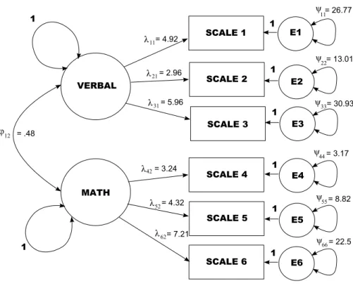
Consider the factor analysis model in Figure 1, which includes six manifest variables, two correlated factors, and a single auxiliary variableV. Though an applied framework is unnec-essary for the example, we may imagine that six scales have been administered to students aged 13 to 18 years, with three of the scales intended to measure verbal ability and three of the scales intended to measure mathematical ability. We assume a measurement invariance violation for the factor loading parameters, whereby the factor loadings for individuals with low values ofV are smaller than the factor loadings for individuals with high values ofV (e.g., factor loadings for older students are larger than those for younger students). We generally wish to assess measurement invariance with respect toV (student age).
5.1. Method
The base factor analysis model, displayed in Figure1with set parameter values, specifies that measurement invariance holds. For the measurement invariance violation, we specify thatV
(student age) impacts the values of verbal factor loadings in the model: if students are 16 through 18 years of age, then the factor loadings corresponding to the first factor (λ11, λ21, λ31)
Figure 1: Path diagram representing the base factor analysis model used for the example and simulations. To induce measurement invariance violations, a seventh observed variable (student age) determines the values of the verbal factor loadings (λ11,λ21,λ31).
reflect those in Figure 1. If students are 13 through 15 years of age, however, then the factor loadings corresponding to the first factor are three standard errors (= asymptotic standard errors divided by√n) lower than those in Figure1. This violation states, e.g., that the verbal ability scales lack measurement invariance with respect to age. For simplicity, we assume that the mathematical scales are invariant.
A sample of size 200 was generated from the model described above, and a test was conducted to examine measurement invariance of the three verbal scales. To carry out the test, a confirmatory factor analysis model (with the paths displayed in Figure1) was fit to the data. Casewise derivatives and the observed information matrix were then obtained, and they were used to calculate the cumulative score process via (13). Finally, we obtained various test statistics and p values from the cumulative score process. These include the double-max statistic from (15), the Cram´er-von Mises statistic from (16), and the maxLM statistic from (17).
As mentioned in the theory section, the tests give us the flexibility to study hypotheses of partial change. That is, we have the ability to test various subsets of parameters. For example, if we suspected that the verbal factor loadings lacked measurement invariance, we could test
H0 : (λi,11 λi,21λi,31) = (λ0,11 λ0,21λ0,31), i= 1, . . . , n, (20) where (λi,11 λi,21 λi,31) represent the verbal factor loading parameters for student i. Thus,
here only k∗ = 3 from the overall k= 19 model parameters (including means) are assessed. Alternatively, we can consider all k∗ = k = 19 parameters, leading to a test of (8). We consider both of these tests below.
5.2. Results
In the results section, we first describe overall results. We then describe estimation of ν and isolation of model parameters violating measurement invariance.
Overall Results
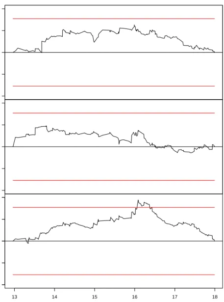
Test statistics for the hypotheses (20) and (8) are displayed in Figure2. Each panel displays a test statistic’s fluctuation across values of student age, with the first column containing tests of (20) and the second column containing tests of (8). The solid horizontal lines represent critical values for α = 0.05, and the Cram´er-von Mises panels also contain a dashed line depicting the value of the test statistic (test statistics for the others are simply the maxima of the processes). In other words, for panels in the first and third rows, (20) is rejected if the process crosses the horizontal line. For panels in the second row, (8) is rejected if the dashed horizontal line is higher than the solid horizontal line.
The figures convey information about several properties of the tests. First, all three tests are more powerful (and in this example significant) if we test only those parameters that are subject to instabilities. Conversely, if all 19 model parameters are assessed (including those that are in fact invariant), the power is decreased. This decrease, however, is less pronounced for the double-max test as it is more sensitive to fluctuations among a small subset of parameters.
Figure3compares the maxLM statistic (solid line) to the maxLRstatistic (dashed line) from (12), as applied to testing (8). The critical values for these two tests are identical, hence the single horizontal line. The figure shows that the two statistics are very similar to one another, with both maxima at the dotted vertical line. This is generally to be expected, because the two tests are asymptotically equivalent. The maxLR statistic cannot be obtained from the empirical fluctuation process, however, so the factor analysis model must be refitted before and after each of the possible threshold valuesν (i.e., here 320 model fits for 160 thresholds).
Estimation of ν and parameter isolation
As described above, the tests of (20) imply that the verbal scales lack measurement invariance. We can also use the tests to: (1) estimate the thresholdν, and (2) isolate specific parameters that violate measurement invariance. For example, as described previously, estimates ofνcan be obtained by examining the peaks in Figure2. For all six panels in the figure, the peaks occur near an age of 16.1. This agrees well with the true threshold of 16.0.
As mentioned previously, the double-max test is advantageous because it yields information about individual parameters violating measurement invariance. That is, it allows us to ex-amine whether or not individual parameters’ cumulative score processes lead one to reject the hypothesis of measurement invariance. Figure 4 shows the individual cumulative score processes for the verbal factor loadings, with the horizontal lines reflecting the critical value at α = 0.05. The figure shows that the third parameter (i.e., λ31) crosses the dashed line, so we would conclude a measurement invariance violation for the third verbal test. The fact
13 14 15 16 17 18 0.0 0.5 1.0 1.5 Age Empir
ical fluctuation process
DM, k* = 3 13 14 15 16 17 18 0 1 2 3 4 5 Age Empir
ical fluctuation process
CvM, k* = 3 14 15 16 17 5 10 15 20 Age Empir
ical fluctuation process
max LM, k* = 3 13 14 15 16 17 18 0.0 0.5 1.0 1.5 Age Empir
ical fluctuation process
DM, k* = 19 13 14 15 16 17 18 0 2 4 6 8 Age Empir
ical fluctuation process
CvM, k* = 19 14 15 16 17 15 20 25 30 35 40 Age Empir
ical fluctuation process
max LM, k* = 19
Figure 2: Three test statistics of (20) (with k∗ = 3) and (8) (with k∗ = 19), based on the example involving measurement invariance with respect to student age. Solid, horizontal lines represent critical values atα = 0.05, and the dotted, horizontal lines (second row) represent values of the Cram´er-von Mises test statistic.
14 15 16 17 0 10 20 30 40 50 Age LR and LM statistics (k* = 19) LR LM
Figure 3: A comparison of the maxLM (solid line) and maxLR (dashed line) test statistics for (8) (i.e., k∗ = 19). The solid horizontal line corresponds to the critical value at α= 0.05 while the dotted vertical line highlights the threshold at which both test statistics assume their maximum.
that the cumulative score process for the first and second loadings did not achieve the critical value represents a Type II error, which implicitly brings into question the tests’ power. This is an example of a situation where the double-max test “wastes” power, as it cannot make use of the fact that multiple model parameters change simultaneously. We generally address the issue of power in the simulations below.
6. Simulation
In this section, we conduct a simulation designed to examine the tests’ power and Type I error rates in the context also employed for the previous example. We examine the power and error rates of three tests: the double-max test, the Cram´er-von Mises test, and the maxLM test. We also compare tests involving only the k∗ = 3 parameters that changed with tests of all k∗ =k= 19 model parameters. The example implied that the former tests had more power, and the simulations provide more detail on the extent to which the tests’ power levels differ. Finally, we also examine the tests’ power across various magnitudes of measurement invariance violations.
−2 −1 0 1 2 λ11 −2 −1 0 1 2 λ21 13 14 15 16 17 18 −2 −1 0 1 2 Age −2 −1 0 1 2 λ31
Figure 4: Cumulative score processes for each verbal factor loadings, with critical values stemming from the double-max test. The solid, horizontal lines correspond to the critical value atα= 0.05.
6.1. Method
Data were generated analogously to the example section. The data were generated from a factor analysis model with two correlated factor and six manifest variables, with individuals with low V (13–15) having smaller factor loadings than individuals with large V (16–18). Sample size and magnitude of measurement invariance violation were manipulated to examine
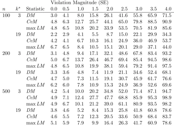
Violation Magnitude (SE) n k∗ Statistic 0.0 0.5 1.0 1.5 2.0 2.5 3.0 3.5 4.0 100 3 DM 3.0 4.1 8.0 15.8 26.1 41.6 55.8 65.9 71.5 CvM 4.8 6.3 12.7 25.7 44.1 65.0 79.8 88.5 90.9 maxLM 4.8 6.5 10.8 20.2 33.9 53.5 70.5 81.9 85.6 19 DM 2.2 2.9 4.1 5.5 8.7 15.0 22.1 29.9 34.3 CvM 4.2 4.1 6.7 10.3 16.1 24.9 36.0 46.9 53.7 maxLM 6.7 6.5 8.4 10.5 15.1 20.1 29.0 37.1 44.0 200 3 DM 3.1 4.8 9.4 17.1 32.1 48.6 67.8 83.4 93.2 CvM 5.0 6.7 13.7 26.4 46.7 69.4 85.4 94.5 98.6 maxLM 4.8 6.5 10.8 19.9 38.1 59.4 79.2 91.4 97.5 19 DM 3.3 3.6 4.8 7.4 11.9 21.1 34.6 52.4 68.1 CvM 4.7 5.0 7.3 11.5 19.1 30.7 45.9 61.7 76.6 maxLM 6.2 6.0 7.8 10.9 15.3 24.9 36.9 52.6 69.6 500 3 DM 4.2 5.4 10.0 20.2 34.8 52.0 71.4 87.1 94.7 CvM 4.9 7.1 12.4 27.7 47.7 68.8 85.9 95.3 98.9 maxLM 4.9 6.7 10.1 21.2 39.0 61.1 80.9 93.5 98.2 19 DM 3.8 4.6 5.2 8.4 15.3 25.8 41.8 60.8 78.6 CvM 4.6 5.5 7.2 12.3 20.5 33.6 50.9 68.4 83.7 maxLM 5.1 5.9 7.9 9.9 16.4 26.3 41.7 60.9 78.6
Table 1: Simulated power for three test statistics across three sample sizesn, nine magnitudes of measurement invariance violations, and two subsets of tested parametersk∗. Abbreviations: CvM = Cram´er-von Mises test; maxLM = Maximum Lagrange multiplier test; DM = Double-max test. See Figure5 for a visualization (using all 17 violation magnitudes).
power: we examined power to detect invariance violations across three sample sizes (n = 100,200,500) and 17 magnitudes of violations. These violations involved the younger students’ values of{λ11, λ21, λ31} deviating from the older students’ values by dtimes the parameters’ asymptotic standard errors (scaled by√n), with d= 0,0.25,0.5, . . . ,4. The 0-standard error condition was used to study Type I error rate.
For each combination of sample size (n) ×violation magnitude (d) ×number of parameters being tested (k∗), 5,000 datasets were generated and tested. In each dataset, half the indi-viduals had “low V” (e.g., 13–15 years of age) and half had “high V” (e.g., 16–18 years of age).
6.2. Results
Full simulation results are presented in Figure 5, and the underlying numeric values for a subset of the results is additionally displayed in Table1. In describing the results, we largely refer to the figure.
Figure 5 displays power curves as a function of violation magnitude, with panels for each combination of sample size (n) × number of parameters being tested (k∗). Separate curves are drawn for the double-max test (solid lines), the Cram´er-von Mises test (dashed lines), and the maxLM (dotted lines). One can generally observe that simultaneous tests of all
Violation Magnitude P o w er 0.2 0.4 0.6 0.8 0 1 2 3 4 k* = 3 n = 100 k* = 19 n = 100 k* = 3 n = 200 0.2 0.4 0.6 0.8 k* = 19 n = 200 0.2 0.4 0.6 0.8 k* = 3 n = 500 0 1 2 3 4 k* = 19 n = 500 CvM max LM DM
Figure 5: Simulated power curves for the double-max test (solid), Cram´er-von Mises test (dashed), and maxLM test (dotted) across three sample sizes n, two subsets of tested pa-rameters k∗, and measurement invariance violations of 0–4 standard errors (scaled by √n). See Table1for the underlying numeric values (using a subset of nine violation magnitudes).
19 parameters result in decreased power, with the tests performing more similarly at the larger sample sizes. The tests distinguish themselves from one another when only the three factor loadings are tested, with the Cram´er-von Mises test having the most power, followed by maxLM, followed by the double-max test. This advantage decreases with increases in
sample size. Table1presents the same results as Figure5, but it is easier to see exact power magnitudes in the table. The table shows that the power advantage of the Cram´er-von Mises test can be as large as 0.1, most notably when three parameters are being tested. It also shows that the Cram´er-von Mises test generally has true Type-I error rates, with the double-max test being somewhat conservative and the maxLM test being slightly liberal.
In summary, we found that the proposed tests have adequate power to detect measurement invariance violations in applied contexts. The Cram´er-von Mises statistic exhibited the best performance for the data generated here, though more simulations are warranted to exam-ine the generality of this finding in other models or other parameter constellations. In the discussion, we describe extensions of the tests in factor analysis and beyond.
7. Discussion
In this paper, we have presented a new family of statistical tests for the study of measurement invariance in psychometrics. The tests, based on stochastic processes, have reasonable power, can isolate subgroups of individuals violating measurement invariance based on a continuous auxiliary variable, and can isolate specific model parameters affected by the violation. In this section, we consider the tests’ use in practice and their extension to more complex scenarios. 7.1. Use in practice
The proposed tests give researchers a new set of tools for studying measurement invariance. For example, they give researchers the flexibility to: (1) simultaneously test all model param-eters, yielding results relevant to many types of measurement invariance (see, e.g.,Meredith 1993), or (2) test a single subset of model parameters, potentially leading to improved power to detect a single type of measurement invariance. The traditional steps have involved hy-pothesizing a specific type of invariance and then testing for it via a LR test, but this is unnecessary under the proposed framework.
In addition to simultaneously testing different types of measurement invariance, the proposed tests allow researchers to easily interpret the nature of the invariance violation. This is made possible through the tests’ abilities to estimate ν, the threshold dividing individuals into subgroups that violate measurement invariance. While a singleν was assumed in this paper, it is also possible to define formal rules for estimating multipleν parameters (seeZeileiset al.
2010). We plan to explore these issues in the future. 7.2. Categorical auxiliary variable
One issue that was largely unaddressed in this paper involved the use of categorical V to study measurement invariance. In this case, groups are already specified in advance, and so traditional methods for fixed subgroups (i.e., LR, Wald, and LM tests) may suffice. Further-more, we can also obtain an LM-type statistic from the framework developed here. Assume the observations are divided intoC categories I1, I2, . . . , IC. Then, the increment of the cu-mulative score process ∆IcB( ˆθ) within each category is just the sum of the corresponding
scores. In somewhat sloppy notation: ∆IcB( ˆθ) = ˆI
−1/2n−1/2X
i∈Ic
This results in aC×k matrix, with one entry for each category-by-model parameter combi-nation. We can test a specific model parameter for invariance by focusing on the associated column of theC×kmatrix and employing a weighted squared sum of the entries in the column to obtain aχ2-distributed statistic with (C−1) degrees of freedom (Hjort and Koning 2002). Alternatively, to simultaneously test multiple parameters, we can sum the χ2 statistics and degrees of freedom for the individual parameters. In addition to categorical V, this frame-work may also be useful for both continuousV with many ties and ordinalV. The number of potential thresholds may be very low in these situations, which impacts the extent to which asymptotic results hold for the main test statistics described in this paper.
7.3. Extensions
The proposed family of tests can be extended in various ways. First, it is possible to construct an algorithm that recursively defines groups of individuals violating measurement invariance with respect to multiple auxiliary variables. Such an algorithm is related to classification and regression trees (Breiman, Friedman, Olshen, and Stone 1984;Merkle and Shaffer 2011; Strobl, Malley, and Tutz 2009), with related algorithms being developed for general parametric models (Zeileis, Hothorn, and Hornik 2008) and Rasch models in particular (Strobl, Kopf, and Zeileis 2010).
Relatedly,S´anchez(2009) describes a general method for partitioning/segmenting structural equation models within a partial least squares framework. This method involves direct maxi-mization of the likelihood ratio (i.e., fitting the model for various subgroups defined byV and choosing the subgroups with the largest likelihood ratio). Thus, unlike the tests described in this paper, this approach does not provide a formal significance test with a controlled level of Type I errors.
The proposed tests also readily extend to other popular psychometric models. Instead of studying measurement invariance in factor analysis, the tests can be used to generally study the stability of structural equation model parameters across observations. For example, it would be possible to assess whether paths between latent variables are stronger for some individuals than for others. Secondly, the tests may be extended to study differential item functioning (DIF) in item response models (e.g., Strobl et al. 2010, who focused on recur-sive partitioning of Rasch models). Traditional DIF methods are similar to those for factor analysis in that subgroups must be specified in advance. While factor-analytic measurement invariance methods and DIF methods have developed largely independently of one another, some treatments (McDonald 1999) and recent research (Stark, Chernyshenko, and Drasgow 2006) have sought to unify the methods. Extensions of the proposed tests can support this endeavor.
7.4. Summary
We have outlined a family of stochastic process-based parameter instability tests from theo-retical statistics and applied them to the issue of measurement invariance in psychometrics. The paper included both theoretical development and study of the tests’ performance. The tests were found to have good properties via simulation, making them useful for many psycho-metric applications. More generally, the tests help solve standing problems in measurement invariance research and provide many avenues for future research, both through extensions of the tests within a factor-analytic context and through application of the tests to new models.
Computational details
All results were obtained using the R system for statistical computing (R Development Core Team 2011), version 2.12.2, employing the add-on packages lavaan 0.4-7 (Rosseel 2011) and OpenMx 0.9.1-1421 (Boker, Neale, Maes, Wilde, Spiegel, Brick, Spies, Estabrook, Kenny, Bates, Mehta, and Fox 2011) for fitting of the factor analysis models and strucchange 1.4-3 (Zeileis, Leisch, Hornik, and Kleiber 2002; Zeileis 2006) for evaluating the parameter in-stability tests. R and the packages lavaan and strucchange are freely available under the General Public License 2 from the Comprehensive R Archive Network at http://CRAN. R-project.org/ while OpenMx is available under the Apache License 2.0 from http:// OpenMx.psyc.virginia.edu/. R code for replication of our results is available at http: //semtools.R-Forge.R-project.org/.
References
Andrews DWK (1993). “Tests for Parameter Instability and Structural Change with Unknown Change Point.”Econometrica,61, 821–856.
Boker S, Neale M, Maes H, Wilde M, Spiegel M, Brick T, Spies J, Estabrook R, Kenny S, Bates T, Mehta P, Fox J (2011). “OpenMx: An Open Source Extended Structural Equation Modeling Framework.”Psychometrika. doi:10.1007/S11336-010-9200-6. Forthcoming. Bollen KA (1989). Structural Equations with Latent Variables. John Wiley & Sons, New
York.
Borsboom D (2006). “When Does Measurement Invariance Matter?” Medical Care, 44(11), S176–S181.
Breiman L, Friedman JH, Olshen RA, Stone CJ (1984). Classification and Regression Trees. Wadsworth, Belmont, CA.
Brown RL, Durbin J, Evans JM (1975). “Techniques for Testing the Constancy of Regression Relationships Over Time.”Journal of the Royal Statistical Society B,37, 149–163.
Hansen BE (1992). “Testing for Parameter Instability in Linear Models.” Journal of Policy Modeling,14, 517–533.
Hansen BE (1997). “Approximate AsymptoticpValues for Structural-Change Tests.”Journal of Business & Economic Statistics,15, 60–67.
Hjort NL, Koning A (2002). “Tests for Constancy of Model Parameters over Time.” Non-parametric Statistics,14, 113–132.
Horn JL, McArdle JJ (1992). “A Practical and Theoretical Guide to Measurement Invariance in Aging Research.”Experimental Aging Research,18, 117–144.
J¨oreskog KG (1971). “Simultaneous Factor Analysis in Several Populations.”Psychometrika, 36, 409–426.
MacCallum RC, Zhang S, Preacher KJ, Rucker DD (2002). “On the Practice of Dichotomiza-tion of Quantitative Variables.”Psychological Methods,7, 19–40.
McDonald RP (1999). Test Theory: A Unified Treatment. Lawrence Erlbaum Associates, Mahwah, NJ.
Meredith W (1993). “Measurement Invariance, Factor Analysis, and Factorial Invariance.” Psychometrika,58, 525–543.
Merkle EC, Shaffer VA (2011). “Binary Recursive Partitioning Methods with Application to Psychology.”British Journal of Mathematical and Statistical Psychology,64(1), 161–181. Millsap RE (2005). “Four Unresolved Problems in Studies of Factorial Invariance.” In
A Maydeu-Olivares, JJ McArdle (eds.), Contemporary Psychometrics, pp. 153–171. Lawrence Erlbaum Associates, Mahwah, NJ.
Nyblom J (1989). “Testing for the Constancy of Parameters over Time.” Journal of the American Statistical Association,84, 223–230.
Ploberger W, Kr¨amer W (1992). “The CUSUM Test with OLS Residuals.” Econometrica, 60(2), 271–285.
R Development Core Team (2011). R: A Language and Environment for Statistical Comput-ing. R Foundation for Statistical Computing, Vienna, Austria. ISBN 3-900051-07-0, URL http://www.R-project.org/.
Rosseel Y (2011). lavaan: Latent Variable Analysis. R package version 0.4-7, URL http: //CRAN.R-project.org/package=lavaan.
S´anchez G (2009). PATHMOX Approach: Segmentation Trees in Partial Least Squares Path Modeling. Ph.D. thesis, Universitat Polit´ecnica de Catalunya.
Satorra A (1989). “Alternative Test Criteria in Covariance Structure Analysis: A Unified Approach.”Psychometrika,54, 131–151.
Shorack GR, Wellner JA (1986). Empirical Processes with Applications to Statistics. John Wiley & Sons, New York, NY.
Stark S, Chernyshenko OS, Drasgow F (2006). “Detecting Differential Item Functioning with Confirmatory Factor Analysis and Item Response Theory: Toward a Unified Strategy.” Journal of Applied Psychology,91, 1292–1306.
Strobl C, Kopf J, Zeileis A (2010). “A New Method for Detecting Differential Item Functioning in the Rasch Model.”Technical Report 92, Department of Statistics, Ludwig-Maximilians-Universit¨at M¨unchen. URLhttp://epub.ub.uni-muenchen.de/11915/.
Strobl C, Malley J, Tutz G (2009). “An Introduction to Recursive Partitioning: Rationale, Application, and Characteristics of Classification and Regression Trees, Bagging, and Ran-dom Forests.” Psychological Methods,14, 323–348.
Wothke W (2000). “Longitudinal and Multi-Group Modeling with Missing Data.” In TD Lit-tle, KU Schnabel, J Baumert (eds.),Modeling Longitudinal and Multilevel Data: Practical Issues, Applied Approaches, and Specific Examples. Lawrence Erlbaum Associates, Mah-wah, NJ.
Zeileis A (2005). “A Unified Approach to Structural Change Tests Based on ML Scores,
F Statistics, and OLS Residuals.”Econometric Reviews,24(4), 445–466.
Zeileis A (2006). “Implementing a Class of Structural Change Tests: An Econometric Com-puting Approach.”Computational Statistics & Data Analysis,50(11), 2987–3008.
Zeileis A, Hornik K (2007). “Generalized M-Fluctuation Tests for Parameter Instability.” Statistica Neerlandica,61, 488–508.
Zeileis A, Hothorn T, Hornik K (2008). “Model-Based Recursive Partitioning.” Journal of Computational and Graphical Statistics,17, 492–514.
Zeileis A, Leisch F, Hornik K, Kleiber C (2002). “strucchange: An R Package for Testing for Structural Change in Linear Regression Models.” Journal of Statistical Software,7(2), 1–38. URLhttp://www.jstatsoft.org/v07/i02/.
Zeileis A, Shah A, Patnaik I (2010). “Testing, Monitoring, and Dating Structural Changes in Exchange Rate Regimes.”Computational Statistics & Data Analysis,54, 1696–1706.
Affiliation: Edgar C. Merkle
Department of Psychology Wichita State University
Wichita, KS 67260-0034, United States of America E-mail: [email protected] URL: http://psychology.wichita.edu/merkle/ Achim Zeileis Department of Statistics Universit¨at Innsbruck Universit¨atsstr. 15
A-6020 Innsbruck, Austria
E-mail: [email protected] URL: http://eeecon.uibk.ac.at/~zeileis/
Recent Paperscan be accessed on the following webpage:
http://eeecon.uibk.ac.at/wopec/
2011-09 Edgar C. Merkle, Achim Zeileis: Generalized measurement invariance
tests with application to factor analysis
2011-08 Michael Kirchler, J¨urgen Huber, Thomas St¨ockl: Thar she bursts
-reducing confusion reduces bubbles modified version forthcoming in
American Economic Review
2011-07 Ernst Fehr, Daniela R¨utzler, Matthias Sutter:The development of
ega-litarianism, altruism, spite and parochialism in childhood and adolescence
2011-06 Octavio Fern´andez-Amador, Martin G¨achter, Martin Larch, Georg
Peter: Monetary policy and its impact on stock market liquidity: Evidence
from the euro zone
2011-05 Martin G¨achter, Peter Schwazer, Engelbert Theurl: Entry and exit of
physicians in a two-tiered public/private health care system
2011-04 Loukas Balafoutas, Rudolf Kerschbamer, Matthias Sutter:
Distribu-tional preferences and competitive behavior forthcoming in
Journal of Economic Behavior and Organization
2011-03 Francesco Feri, Alessandro Innocenti, Paolo Pin:Psychological pressure
in competitive environments: Evidence from a randomized natural experiment: Comment
2011-02 Christian Kleiber, Achim Zeileis: Reproducible Econometric Simulations
2011-01 Carolin Strobl, Julia Kopf, Achim Zeileis: A new method for detecting
differential item functioning in the Rasch model
2010-29 Matthias Sutter, Martin G. Kocher, Daniela R¨utzler and Stefan
T. Trautmann: Impatience and uncertainty: Experimental decisions predict
adolescents’ field behavior
2010-28 Peter Martinsson, Katarina Nordblom, Daniela R¨utzler and
Matt-hias Sutter: Social preferences during childhood and the role of gender and
age - An experiment in Austria and Sweden Revised version forthcoming in
Economics Letters
2010-27 Francesco Feri and Anita Gantner: Baragining or searching for a better
price? - An experimental study. Revised version accepted for publication in
2010-25 Jes´us Crespo-Cuaresma and Octavio Fern´andez Amador: Business cycle convergence in EMU: A second look at the second moment
2010-24 Lorenz Goette, David Huffman, Stephan Meier and Matthias Sutter:
Group membership, competition and altruistic versus antisocial punishment: Evidence from randomly assigned army groups
2010-23 Martin G¨achter and Engelbert Theurl:Health status convergence at the
local level: Empirical evidence from Austria (revised Version March 2011)
2010-22 Jes´us Crespo-Cuaresma and Octavio Fern´andez Amador: Buiness
cycle convergence in the EMU: A first look at the second moment
2010-21 Octavio Fern´andez-Amador, Josef Baumgartner and Jes´us
Crespo-Cuaresma: Milking the prices: The role of asymmetries in the price
trans-mission mechanism for milk products in Austria
2010-20 Fredrik Carlsson, Haoran He, Peter Martinsson, Ping Qin and
Matt-hias Sutter: Household decision making in rural China: Using experiments
to estimate the influences of spouses
2010-19 Wolfgang Brunauer, Stefan Lang and Nikolaus Umlauf:Modeling
hou-se prices using multilevel structured additive regression
2010-18 Martin G¨achter and Engelbert Theurl:Socioeconomic environment and
mortality: A two-level decomposition by sex and cause of death
2010-17 Boris Maciejovsky, Matthias Sutter, David V. Budescu and Patrick
Bernau: Teams make you smarter: Learning and knowledge transfer in
auc-tions and markets by teams and individuals
2010-16 Martin G¨achter, Peter Schwazer and Engelbert Theurl: Stronger sex
but earlier death: A multi-level socioeconomic analysis of gender differences in mortality in Austria
2010-15 Simon Czermak, Francesco Feri, Daniela R¨utzler and Matthias
Sut-ter:Strategic sophistication of adolescents - Evidence from experimental
normal-form games
2010-14 Matthias Sutter and Daniela R¨utzler: Gender differences in competition
emerge early in live
2010-13 Matthias Sutter, Francesco Feri, Martin G. Kocher, Peter
Martins-son, Katarina Nordblom and Daniela R¨utzler: Social preferences in
efficiency of policy interventions
2010-11 Alexander Strasak, Nikolaus Umlauf, Ruth Pfeifer and Stefan Lang:
Comparing penalized splines and fractional polynomials for flexible modeling of the effects of continuous predictor variables
2010-10 Wolfgang A. Brunauer, Sebastian Keiler and Stefan Lang: Trading
strategies and trading profits in experimental asset markets with cumulative information
2010-09 Thomas St¨ockl and Michael Kirchler: Trading strategies and trading
profits in experimental asset markets with cumulative information
2010-08 Martin G. Kocher, Marc V. Lenz and Matthias Sutter: Psychological
pressure in competitive environments: Evidence from a randomized natural experiment: Comment
2010-07 Michael Hanke and Michael Kirchler: Football Championships and
Jer-sey sponsors’ stock prices: An empirical investigation
2010-06 Adrian Beck, Rudolf Kerschbamer, Jianying Qiu and Matthias
Sut-ter: Guilt from promisebreaking and trust in markets for expert services
-Theory and experiment
2010-05 Martin G¨achter, David A. Savage and Benno Torgler: Retaining the
thin blue line: What shapes workers’ intentions not to quit the current work environment
2010-04 Martin G¨achter, David A. Savage and Benno Torgler:The relationship
between stress, strain and social capital
2010-03 Paul A. Raschky, Reimund Schwarze, Manijeh Schwindt and
Fer-dinand Zahn: Uncertainty of governmental relief and the crowding out of
insurance
2010-02 Matthias Sutter, Simon Czermak and Francesco Feri: Strategic
sophi-stication of individuals and teams in experimental normal-form games
2010-01 Stefan Lang and Nikolaus Umlauf: Applications of multilevel structured
Working Papers in Economics and Statistics
2011-09
Edgar C. Merkle, Achim Zeileis
Generalized measurement invariance tests with application to factor analysis
Abstract
The issue of measurement invariance commonly arises in factor-analytic contexts, with methods for assessment including likelihood ratio tests, Lagrange multiplier tests, and Wald tests. These tests all require advance definition of the number of groups, group membership, and offending model parameters. In this paper, we con-struct tests of measurement invariance based on stochastic processes of casewise derivatives of the likelihood function. These tests can be viewed as generalizations of the Lagrange multiplier test, and they are especially useful for: (1) isolating spe-cific parameters affected by measurement invariance violations, and (2) identifying subgroups of individuals that violated measurement invariance based on a conti-nuous auxiliary variable. The tests are presented and illustrated in detail, along with simulations examining the tests’ abilities in controlled conditions.
ISSN 1993-4378 (Print) ISSN 1993-6885 (Online)