Bilinear Model Predictive Control of a
HVAC System Using Sequential Quadratic
Programming
Anthony Kelman∗ Francesco Borrelli∗∗
∗Department of Mechanical Engineering, University of California, Berkeley, CA 94720-1740 USA (e-mail: [email protected]) ∗∗Department of Mechanical Engineering, University of California,
Berkeley, CA 94720-1740 USA (e-mail: [email protected])
Abstract:We study the problem of heating, ventilation, and air conditioning (HVAC) control in a typical commercial building. We propose a model predictive control (MPC) approach which minimizes energy use while satisfying occupant comfort constraints. A sequential quadratic programming algorithm is used to efficiently solve the resulting bilinear optimization problem. This paper presents the control design approach and the procedure for computing its solution. Extensive numerical simulations show the effectiveness of the proposed approach. In particular, the MPC is able to systematically reproduce a variety of well-known commercial solutions for energy savings, which include demand response, “economizer mode” and precooling/preheating.
1. INTRODUCTION
The building sector consumes about 40% of the energy used in the United States and is responsible for nearly 40% of greenhouse gas emissions, see McQuade (2009). It is therefore economically, socially and environmentally significant to reduce the energy consumption of buildings. Previous work by Henze et al. (2004); Ma et al. (2010); Oldewurtel et al. (2010) has evaluated the energy saving potential of model predictive control (MPC) for heating ventilation and air conditioning (HVAC) in buildings. The main idea of MPC is to use a model of the plant to predict the future evolution of the system, see Borrelli (2003); Mayne et al. (2000). At each discrete sampling time, an open-loop optimal control problem is solved over a finite horizon starting from the current state. The optimal command signal is applied to the process only during the first sampling interval. At the next time step a new optimal control problem based on new measurements of the state is solved over a shifted horizon. Model predictive control has become the accepted standard in the process industry for solving complicated constrained multivariable control problems, see Qin and Badgwell (2003). The success of MPC is largely due to its ability to simply and effectively handle hard constraints on states and control inputs. Section 2 of this paper introduces the common type of HVAC system we focus on, then derives low-order models for the temperature dynamics and energy costs. Section 3 outlines the MPC control algorithm and presents a tailored sequential quadratic programming (SQP) method which exploits the bilinear structure of the optimal control problem. Simulation results presented in Section 4 show good performance and computational tractability of the resulting scheme. Additionally, the model predictive con-troller exhibits desirable control behaviors that resemble modern advanced heuristic strategies for HVAC control, reproducing those strategies in a systematic manner.
2. SYSTEM MODEL
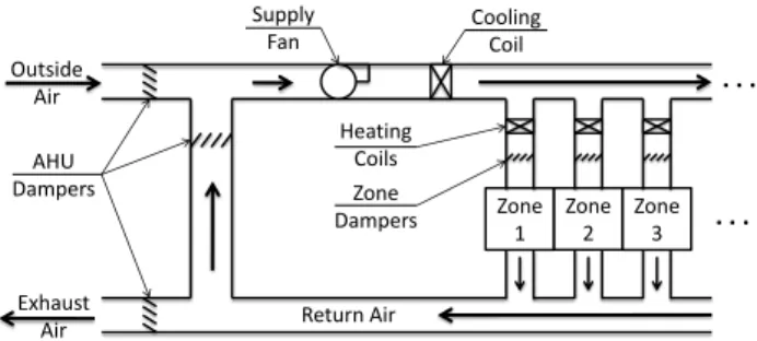
The system considered in this work, known as variable air volume (VAV) with reheat, is depicted in Fig. 1. This type of HVAC system provides cooling using a variable speed supply fan and a cooling coil (water-to-air heat exchanger) located in a central air handling unit (AHU). A cold water valve controls the cooling coil outlet air to a setpoint temperature, and the supply fan distributes the cold air to every thermal zone served by the same AHU. The AHU supply fan speed determines the total flow rate to all zones. The supply air flows from the AHU into each thermal zone through a “VAV box” which consists of a damper and a heating coil. The damper regulates the flow rate to the thermal zone and the heating coil reheats the supply air to a higher temperature, if required.
Return Air Supply Fan Zone 1 AHU Dampers Cooling Coil Heating Coils Zone Dampers . . . Zone 2 Zone 3 . . . Outside Air Exhaust Air
Fig. 1. VAV with reheat HVAC system schematic
The mixed exit air from all zones recirculates back to the AHU through a return duct. A set of dampers in the AHU controls the mix of outside ambient and recirculated air used as the source for supply air. Usually the return air will be cooler than ambient temperature on a hot day when cooling is required, or warmer than ambient on a cold day when heating is required. So conventional practice is to
recirculate as much air as possible, while maintaining a minimum fraction of fresh air for acceptable indoor air quality. However, the opposite scenario of cooling when return air is warmer than ambient (or heating when return air is cooler than ambient) can occur, and in that case using 100% outside air consumes the least total coil energy. This is known as “economizer” operation.
In order to develop a low-order control-oriented building thermal model, we make the following assumptions.
A1 The average air temperature dynamics of the thermal zones can be reasonably approximated as first-order. We therefore combine the thermal capacitance of the air, walls, furnishings, etc. of zoneiis combined into a single lumped parameter denoted (mc)i.
A2 Humidity is not explicitly modeled.1
A3 All dynamics except those of the thermal zones are neglected. Actuators are assumed to instantly meet their control setpoints.
A4 Predictions of outside ambient temperatureToa and
the thermal loads ˙Qi in each zone due to occupants,
equipment, and all heat transfer to or from ambient and other zones are known in advance.2
2.1 Zone Temperature Dynamics
A first order energy balance gives the following continuous time system dynamics for the temperatureTzi of zonei.
(mc)i
d
dtTzi= ˙Qi+ ˙mzicp(Tsi−Tzi). (1) where cp is the specific heat capacity of air, and the
control inputs are the mass flow rates ˙mzi and supply
temperaturesTsi to each zone.
If we neglect heat transfer by radiation, the thermal loads ˙
Qi are an affine function of the zone temperatures,
˙ Q= ˙ Q1 .. . ˙ Qn =R Tz1 .. . Tzn + ˙Qoffset,
wherenis the number of thermal zones served by the same AHU,Ris a symmetricn×nmatrix and ˙Qoffsetis ann×1
time-varying vector. The elements ofR are given by
Rij = UAij i6=j −UAoi− i−1 X k=1 UAik− n X k=i+1 UAik i=j
where UAij =UAji is the heat transfer coefficient times
area between zonesiandj. Zoneiand zonejhave no heat transfer between them when UAij =UAji = 0. The heat
transfer coefficient times area between zoneiand specified external temperatures (such asToa) is denotedUAoi. 1 Humidity and latent heat can be important factors affecting HVAC design and actual energy use, but they are not typically directly measured or controlled. We will deal with this thermodynamic sim-plification indirectly: throughout this entire work, every temperature is meant to represent an equivalent dry air temperature, i.e. the temperature at which dry air would have the same specific enthalpy as the actual moist air mixture.
2 This is a strong assumption, since load and weather predictions are not perfectly accurate. We are investigating extensions of this MPC scheme to robustly account for prediction and model uncertainty.
We can use a weighted undirected graph representation in order to describe the coupling between zones. In that case, −R is equal to the weighted Laplacian matrix of the zone connectivity graph plus a diagonal matrix.
The compact form of (1) for all zones together is then M d
dtTz=R Tz+ ˙Qoffset+cpm˙z◦(Ts−Tz), (2) where M = diag((mc)1, . . . ,(mc)n), Tz = [Tz1, . . . , Tzn]0,
˙
mz = [ ˙mz1, . . . ,m˙zn]0, Ts = [Ts1, . . . , Tsn]0, and◦ denotes
the elementwise product.
Assuming ˙mzandTsare zero-order held at sample rate ∆t,
we discretize (2) using the trapezoidal method to obtain MT + z −Tz ∆t =R T+ z +Tz 2 + ˙ Q+offset+ ˙Qoffset 2 (3) +cpm˙z◦ Ts− Tz++Tz 2 , where T+ z and ˙Q +
offset denote the corresponding values at
the next discrete time stept+ ∆t. We choose the trape-zoidal discretization as a compromise between simplicity and stability (which some methods lack when ∆tis large).
2.2 Air Handling Unit Model
Although we have neglected the dynamics of the AHU, we must introduce additional control inputs and constraints to capture recirculation behavior and the energy cost.
Table 1. Additional variables for AHU model
Symbol Description Units
dr Fraction of supply flow
recirculated from zones dimensionless
Tr Temperature of mixed
return air from zones
◦C
Tm inlet air temperatureAHU cooling coil ◦C
Tc AHU cooling coil outlet
air temperature setpoint
◦C
Assuming there is no heat loss or gain in the return duct, Tris a flow-weighted average of the zone temperatures,
Tr= Pn i=1( ˙mziTzi) Pn i=1m˙zi . (4)
An energy balance of the AHU then gives
Tm= (1−dr)Toa+drTr. (5) 2.3 Cost Function
We will consider energy use of the cooling and heating coils in terms of air-side thermal power, which we can directly calculate from the models in the previous section. We represent all of the operating characteristics of the cold and hot water circuits with two constant parameters: efficiencyηhfor the hot side, and coefficient of performance
ηcfor the cold side. So power used by the heating coils and
cooling coil are given respectively byPh andPc where
Ph= cp ηh n X i=1 ( ˙mzi(Tsi−Tc)), (6) andPc= cp ηc n X i=1 ˙ mzi ! (Tm−Tc). (7)
Remark 1. A higher-fidelity model would include ancillary equipment such as water pumps and cooling towers, and a detailed water-side energy balance.
The electrical powerPf used by the supply fan is equal to
Pf = n X i=1 ˙ mzi ! ∆p ρ ηf ,
where ∆p is the pressure difference across the fan, ρ is the air density, and ηf is the efficiency of the fan. If all
zone dampers were held at fixed positions, incompressible flow would give ∆p ∝ (P
˙
mzi)2. However, when zone
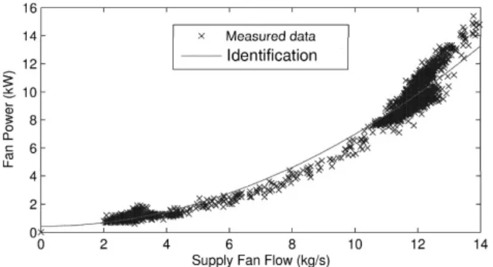
dampers open, the pressure drop for a given flow rate decreases. As an average trend direction, increasing total flow will correspond to more-open zone dampers. So we expect pressure drop to increase more slowly than total flow squared. For simplicity we restrict our model to polynomial form, so we take ∆p=ρ ηfκfPm˙zi. Recorded
data for a representative AHU supply fan shows in Fig. 2 that fan power versus fan flow fits a quadratic model.
Fig. 2. Recorded data from an AHU supply fan in the Bancroft Library at University of California, Berkeley With this form of fit and simplification, we have
Pf =κf n X i=1 ˙ mzi !2 , (8)
where κf is a parameter that captures both the fan
efficiency and the duct pressure losses.
We introduce several parameters to reflect utility pricing. The cost in currency per unit energy content is denoted re for electricity andrh for heating fuel (typically gas, or
steam from a central plant). These costs may vary in time, especially for electricity, to reflect time-of-use or dynamic utility pricing. We assume time variation of utility rates occurs in a zero-order hold manner at sample rate ∆t. We also incorporate a feature of some utility structures wherein peak electric power use is penalized. Some utilities only implement this peak-use charge during certain hours of the day, so we express this feature by defining a windowing functionφ(t). The value ofφ(t) equals the given cost per unit peak power during restricted time intervals, and zero elsewhere.
Assuming cold water is produced immediately on demand by electric chillers, and likewise for hot water by a fuel-powered boiler or district steam heat exchanger, the total utility cost from timet to timet+N∆tis
J = Z t+N∆t t (rePf+rePc+rhPh)dτ + max τ∈[t,t+N∆t] (φ(τ)(Pf+Pc)), (9)
whereN is the prediction horizon length.
Note that the cooling coil power (7) depends on the cooling coil inlet air temperatureTm, which depends (5)
on return air temperatureTr, which depends (4) on zone
temperaturesTz, so this utility cost integral is a function
of the state variables and all of the control inputs. The integral in (9) is approximated numerically according to the trapezoidal discretization for consistency with the discrete state dynamics (3).
2.4 Constraints
The system states and control inputs are subject to the following constraints due to control requirements and actuator limits.
C1: Tzi≤Tzi≤Tzi ∀i∈ {1, . . . , n}, comfort range.
C2: ˙mzi ≤m˙zi≤m˙zi ∀i∈ {1, . . . , n}, minimum
ventila-tion requirement and maximum VAV box capacity. C3: Tsi ≥ Tc ∀ i ∈ {1, . . . , n}, heating coils can only
increase temperature.
C4: Tsi≤Th ∀i∈ {1, . . . , n}, heating coil capacity.
C5: Tc≤Tm, cooling coil can only decrease temperature.
C6: Tc≥Tc, cooling coil capacity.
C7: 0≤dr≤dr, minimum is no recirculation, maximum
set by required fresh air for indoor air quality. In all of the above constraints, limit values denoted by ? and?may be time-varying and are assumed to be known in advance. These constraints must hold at all timest. Due to the trapezoidal discretization of the system dy-namics, we approximate the time variation of the zone temperaturesTzias piecewise linear between discrete time
stepstandt+ ∆t. We treat the disturbance inputs ˙Qoffset
and Toa the same way, as continuous piecewise linear
functions of time. All of the control inputs are zero-order held so they are discontinuous piecewise constant functions of time. Due to (5), cooling coil inlet temperature Tm
is therefore discontinuous and piecewise linear in time. To enforce constraint C5 at all times we introduce the following additional variables
e Tr= Pn i=1( ˙mziTzi+) Pn i=1m˙zi , (10) e Tm= (1−dr)Toa++drTer, (11) e Pc= cp ηc n X i=1 ˙ mzi ! (Tem−Tc), (12)
and corresponding constraint C8: Tc≤Tem.
Multiply both sides of (4) and (10) byPm˙
zi: n X i=1 ˙ mzi ! Tr= n X i=1 ( ˙mziTzi), (13) n X i=1 ˙ mzi ! e Tr= n X i=1 ( ˙mziTzi+). (14)
Note that whenPm˙
zi = 0, the HVAC system consumes
no energy and the system dynamics evolve only according to thermal loads ˙Qi. In that case the return temperature
is not important, so enforcing (13) and (14) is equivalent for our purposes to enforcing (4) and (10).
3. OPTIMAL CONTROL FORMULATION Let xk|t be the value of the state vector Tz at time
t +k∆t predicted at time t, uk|t be the value of the
combined control input vector [ ˙m0z, Ts0, dr, Tc]0 at timet+
k∆t predicted at time t, and vk|t be the value of the
vector of auxiliary variables [Tr, Tm, Ph, Pc, Pf,Ter,Tem,Pec]0
at time t+k∆tpredicted at timet.
The system dynamics (3), and auxiliary-variable equalities (5)-(8) and (11)-(14) can all be expressed in the following bilinear form. 1 2 xk|t uk|t vk|t xk+1|t 0 Cj,k|t xk|t uk|t vk|t xk+1|t +d 0 j,k|t xk|t uk|t vk|t xk+1|t +ej,k|t= 0 ∀j ∈ {1, . . . , n+nv}, ∀ k∈ {0, . . . , N−1} (15)
The matrices Cj,k|t are symmetric and indefinite, and
nv= 8 is the number of auxiliary variables.
We cannot influence whether the given initial conditions x0|t = Tz(t) satisfy the comfort constraints C1, so we
compactly represent the constraints C1-C8 as Ak|t uk|t vk|t xk+1|t ≤bk|t, ∀ k∈ {0, . . . , N−1}. (16)
Letrk|t be the value of the vector [0,0, rh,r2e, re,0,0,r2e]0
at time t+k∆t. Then by the trapezoidal discretization, Z t+N∆t t (rePf+rePc+rhPh)dτ = N−1 X k=0 ∆t rk|t0 vk|t. (17)
Lastly, we introduce an epigraph variable βt to represent
the peak power term in (9). LetFk|t= 0 0 0 φ(τ) φ(τ) 0 0 0 0 0 0 0 φ(τ) 0 0 φ(τ) evaluated at τ =t+k∆t. Then we have the equivalence that
max τ∈[t,t+N∆t] (φ(τ)(Pf+Pc)) = minβt s.t.Fk|tvk|t≤ βt βt , ∀k∈ {0, . . . , N−1}. (18) The constrained finite time optimal control (CFTOC) problem at time tis then
min Xt,Ut,Vt,βt βt+ N−1 X k=0 ∆t rk|t0 vk|t (19) s.t,∀j∈ {1, . . . , n+nv}, ∀k∈ {0, . . . , N−1}, 1 2 xk|t uk|t vk|t xk+1|t 0 Cj,k|t xk|t uk|t vk|t xk+1|t +d 0 j,k|t xk|t uk|t vk|t xk+1|t +ej,k|t= 0 Ak|t uk|t vk|t xk+1|t ≤bk|t, Fk|tvk|t≤ 1 1 βt, x0|t=Tz(t)
where Ut = {u0|t, . . . , uN−1|t} is the set of predicted
control inputs at time t, Xt ={x1|t, . . . , xN|t} is the set
of predicted system states at timet, starting from initial statex0|t=Tz(t) and applying the input sequence Ut to
the system model (3), and Vt ={v0|t, . . . , vN−1|t} is the
corresponding set of predicted auxiliary variables att. Let the optimal solution of problem (19) have input sequence denoted by U?
t = {u?0|t, . . . , u ?
N−1|t}. Then, the
first step of U?
t is input to the system, u(t) = u?0|t. The
optimization (19) is repeated at time t + ∆t, with the updated new state
x0|t+∆t=Tz(t+ ∆t)
yielding amoving or receding horizon control strategy. The values ofbk|t+∆t,dj,k|t+∆t,ej,k|t+∆t, Fk|t+∆t, andrk|t+∆t
may change relative to the previous time step due to time-varying constraints, predictions, and utility costs.
3.1 Sequential Quadratic Programming Approach
The optimization problem (19) is nonconvex due to the nonlinear equality constraints (15). The method of se-quential quadratic programming (SQP) is applied here by linearizing (15) and adding a convex quadratic term to the cost that approximates the Hessian of the Lagrangian function, see Han (1977); Nocedal and Wright (2006). Let λj,k|t be the Lagrange multiplier corresponding to
equality constraint j of step k in problem (19) at time t. The Hessian of the Lagrangian of problem (19) is then
n+nv X j=1 0n×(n+nu+nv)N I(n+nu+nv)N 0 λj,0|tCj,0|t 0 0 0 0n×(n+nu+nv)N I(n+nu+nv)N + N−1 X k=1 "0( n+nu+nv)k−n 0 0 0 λj,k|tCj,k|t 0 0 0 0(n+nu+nv)(N−k−1) #! (20) where nu = 2n+ 2 is the number of control inputs. The
firstnrows and firstncolumns ofCj,0|tfor constraints at
time stepk= 0 are removed because the initial state x0|t
is a known quantity. Since each matrixCj,k|tis indefinite, this exact Hessian of the Lagrangian is also indefinite. We can efficiently calculate the smallest eigenvalue and corresponding eigenvector of this Hessian using an Arnoldi iteration, see Lehoucq et al. (1998). We construct a posi-tive semidefinite approximation of the Hessian by adding a multiple of the identity to (20). Using the available second derivative information in this manner was observed to reduce the number of iterations required for convergence relative to the quasi-Newton approaches of the commercial SQP routines we tested.
4. SIMULATION RESULTS
We present simulation results for the following cases: (1) Nominal case, re uses “low” value from Table 2 and
φ(t) = 0 at all times.
(2) Modified electric rate schedule:re uses “high” value
between 12 noon and 4:30 PM and the “low” value at all other times. No peak power charge, φ(t) = 0. (3) Peak power charge:φ(t) = 1 $/kW andreuses “low”
Table 2. Parameter values used
Parameter Value Units
n 5 zones N 48 steps ∆t 1800 s cp 1 kJ/(kg·K) (mc)i 1000 kJ/K R 0 kW/K ηh 0.9 dimensionless ηc 4 dimensionless κf 0.065 kW·s2/kg2 re n“high” = 1.5·10−4 “low” = 3·10−5 $/kJ rh 5·10−6 $/kJ T0 18 ◦C Tzi n6:30 AM to 6:30 PM = 21 7 PM to 6 AM = 12 ◦C Tzi n6:30 AM to 6:30 PM = 24 7 PM to 6 AM = 32 ◦C ˙ mzi n6:30 AM to 6:30 PM = 0.025 7 PM to 6 AM = 0 kg/s ˙ mzi 1.5 kg/s Tc 5 ◦C Th 40 ◦C dr 0.9 dimensionless
For ambient temperature Toa, we use a sinusoid with
period 1 day, minimum value 10◦C at time 1:30 AM, and maximum value 30◦C at 1:30 PM. Zone thermal loads ˙Qi
are set to the time-varying profiles shown in Fig. 3.
00:00 06:00 12:00 18:00 00:00 −2 −1 0 1 2 3
Zone Thermal Load (kW)
Time (hh:mm) Zones 1−4 Zone 5
Fig. 3. Zone thermal loads ˙Qi
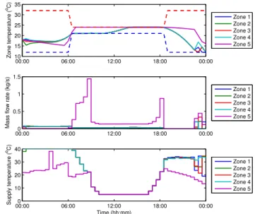
The SQP iterations were computed using the solver BPMPD, see M´esz´aros (1996). The results of case 1 are shown in Fig. 4 and 5, case 2 is shown in Fig. 6, and case 3 is shown in Fig. 7. More extensive parametric simulations were executed but are not included here due to space constraints. Those results can be found in a technical report available athttp://www.mpc.berkeley.edu/. We observe several interesting behaviors for the nominal case 1 in Fig. 4 and 5. Before the occupied period begins at 6:30 AM, zone 5 is set to zero flow and zones 1-4 have a small flow rate at the maximum heating temperature to counteract the cooling loads (negative ˙Qi). All zones
preheat to satisfy the tighter occupied temperature con-straints before the occupied hours begin. From 6:30 AM until 9 AM, zone 5 is in cooling mode but the other zones are in heating. This period is an economizer mode condi-tion: a mix of outside air maintains the mixed temperature close toTzi, while zone 5 satisfies its cooling demand with a very large flow rate. After 9 AM the ambient tempera-ture is warmer than the return temperatempera-ture so the AHU dampers return to maximum recirculation. The cooling
00:00 06:00 12:00 18:00 00:00 10 15 20 25 30 35 Zone temperature ( oC) Zone 1 Zone 2 Zone 3 Zone 4 Zone 5 00:000 06:00 12:00 18:00 00:00 0.5 1 1.5
Mass flow rate (kg/s)
Zone 1 Zone 2 Zone 3 Zone 4 Zone 5 00:000 06:00 12:00 18:00 00:00 10 20 30 40 Time (hh:mm) Supply temperature ( oC) Zone 1 Zone 2 Zone 3 Zone 4 Zone 5
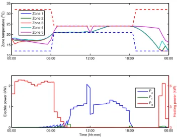
Fig. 4. Case 1 zone results. Shown dashed in the first plot areTzi andTzi. 00:00 06:00 12:00 18:00 00:00 10 20 30 Temperature ( oC) 0 0.5 1 Recirculation fraction Toa Tm Tr dr 00:000 06:00 12:00 18:00 00:00 10 20 30 Temperature ( oC) Tc Tm 00:000 06:00 12:00 18:00 00:00 1 2 Time (hh:mm) Electric power (kW) 0 3 6 Heating power (kW) Pc Pf Ph
Fig. 5. Case 1 AHU results.
coil activates at this time, reaching its lowest setpoint by 10AM. Zones 1-4 begin transitioning to cooling mode here. Immediately before the end of the occupied period at 6:30 PM, we see a cooling coil supply temperature reset behavior. The load prediction is much lower after 6:30 PM, so the cooling coil begins increasing its setpoint early, trading lower cooling power for higher fan power (the flow to zone 5 must increase to keep it cooled using warmer supply air). The erratic one-at-a-time heating of zones 1-4 after 10:30 PM appears to be a consequence of the return temperature dependence on mass flows. When only one zone is heated with a large mass flow (others at low flow), the return temperature is influenced most by the heated zone. Increased return temperature reduces the required heating coil energy for the next zones to be heated. Both case 2 in Fig. 6 and case 3 in Fig. 7 demonstrate precooling of zone 5 and lengthened cooling of zones 1-4, but with different timing and intent. In case 2, φ(t) = 0 but the electric raterehas a higher value between 12 noon
and 4:30 PM. So precooling is only performed immediately before noon, with a corresponding spike in cooling power,
so that less cooling energy is used between 12 noon and 4:30 PM. In case 3, φ(t) = 1 so load-shifting is used to minimize peak power. Zone 5 is precooled beginning earlier in the morning, increasing cooling power at a time when it would otherwise be low and shifting electric power use away from the times it would normally be highest. Our computational results show that in response to either time-varying electric rates (re, case 2) or peak power
charges (φ(t), case 3), this optimization-based controller does not use appreciably more total energy. We are not showing the combination ofrehigh andφ(t) = 1 here, but
the results are very similar to case 3. Imposing a charge on peak power rules out the type of short-duration precooling seen in case 2. 00:00 06:00 12:00 18:00 00:00 10 15 20 25 30 35 Zone temperature ( oC) Zone 1 Zone 2 Zone 3 Zone 4 Zone 5 00:000 06:00 12:00 18:00 00:00 1 2 Time (hh:mm) Electric power (kW) 0 3 6 Heating power (kW) Pc Pf Ph
Fig. 6. Case 2 overview. Note the precooling and spike in cooling power immediately before noon.
00:00 06:00 12:00 18:00 00:00 10 15 20 25 30 35 Zone temperature ( oC) Zone 1 Zone 2 Zone 3 Zone 4 Zone 5 00:000 06:00 12:00 18:00 00:00 1 2 Time (hh:mm) Electric power (kW) 0 3 6 Heating power (kW) Pc Pf Ph
Fig. 7. Case 3 overview. Note the timing of the precooling and the intentional plateau in cooling power.
5. CONCLUSIONS
This MPC algorithm has shown encouraging results in a few interesting cases for a sample problem. The control performance, entirely from an optimization origin, exhibits aspects of heuristic HVAC control such as economizer
control, supply temperature reset, demand response, pre-cooling, and load-shifting in a coordinated manner. The computational time for each of the above cases was less than one minute, faster than the time scales of a HVAC system. We are working toward real-time receding-horizon implementation of this algorithm to experimentally con-trol a building. Future work is necessary in the areas of system identification, model validation, and thermal load prediction. We also plan on investigating robust MPC for this system, wherein we account for uncertainty in future thermal load values and the effects of model mismatch. Lastly, the SQP algorithm only guarantees local solu-tions to non-convex nonlinear optimization problems, so we are investigating branch-and-bound extensions of this approach for global search algorithms.
ACKNOWLEDGEMENTS
This work was supported by the Department of Energy under grant number ???. We thank Allan Daly and Yudong Ma for discussions regarding HVAC modeling and opti-mization.
REFERENCES
Borrelli, F. (2003).Constrained Optimal Control of Linear and Hybrid Systems, volume 290. Springer-Verlag. Han, S. (1977). A globally convergent method for
nonlin-ear programming. Journal of Optimization Theory and Applications, 22(3), 297 – 309.
Henze, G., Felsmann, C., and Knabe, G. (2004). Evalu-ation of optimal control for active and passive building thermal storage. International Journal of Thermal Sci-ences, 43(2), 173 – 183.
Lehoucq, R., Sorensen, D., and Yang, C. (1998).ARPACK users’ guide: solution of large-scale eigenvalue problems with implicitly restarted Arnoldi methods. SIAM Publi-cations.
Ma, Y., Borrelli, F., Hencey, B., Coffey, B., Bengea, S., and Haves, P. (2010). Model predictive control for the operation of building cooling systems. In2010 American Control Conference, 5106 – 5111.
Mayne, D., Rawlings, J., Rao, C., and Scokaert, P. (2000). Constrained model predictive control: Stability and op-timality. Automatica, 36(6), 789 – 814.
McQuade, J. (2009). A systems approach to high perfor-mance buildings. Technical report, United Technolo-gies Corporation. http://gop.science.house.gov/
Media/hearings/energy09/april28/mcquade.pdf.
M´esz´aros, C. (1996). Fast cholesky factorization for inte-rior point methods of linear programming. Computers & Mathematics with Applications, 31(4-5), 49 – 54. Nocedal, J. and Wright, S.J. (2006). Numerical
Optimiza-tion, chapter 18. Springer-Verlag.
Oldewurtel, F., Parisio, A., Jones, C., Morari, M., Gyalis-tras, D., Gwerder, M., Stauch, V., Lehmann, B., and Wirth, K. (2010). Energy efficient building climate control using stochastic model predictive control and weather predictions. In 2010 American Control Con-ference, 5100 – 5105.
Qin, S. and Badgwell, T. (2003). A survey of industrial model predictive control technology. Control Engineer-ing Practice, 11, 733 – 764.