Gauge engineering and propagators
Axel Maas1,a
1Institute of Physics, NAWI Graz, University of Graz, Universitätsplatz 5, A-8010 Graz, Austria
Abstract.Beyond perturbation theory gauge-fixing becomes more involved due to the Gribov-Singer ambiguity: The appearance of additional gauge copies requires to define a procedure how to handle them. For the case of Landau gauge the structure and properties of these additional gauge copies will be investigated. Based on these properties gauge conditions are constructed to account for these gauge copies.
The dependence of the propagators on the choice of these complete gauge-fixings will then be investigated using lattice gauge theory for Yang-Mills theory. It is found that the implications for the infrared, and to some extent mid-momentum behavior, can be substantial. In going beyond the Yang-Mills case it turns out that the influence of matter can generally not be neglected. This will be briefly discussed for various types of matter.
1 Introduction
The determination of the gauge-dependent correlation functions, especially propagators and vertices, is a long-standing challenge [1–6]. One of the main problems is that the concept of a gauge itself becomes more involved beyond perturbation theory. The reason for this is the appearance of the Gribov-Singer ambiguity, essentially the presence of perturbatively absent additional gauge copies. This obstructs any perturbative gauge-fixing from being complete, i. e. able to fully specify how the gauge orbit should be sampled [7, 8]. Thus, extended sampling prescriptions are necessary to provide well-defined gauges.
While formulating complete gauge fixings is possible in principle, the remaining practical obstacle
is to find such prescriptions which can be implemented in different methods. The motivation for such
comparisons of gauge-dependent, rather than gauge-invariant, quantities is that none of the available non-perturbative methods is truly exact. A comparison of results at the level of gauge-dependent quantities has turned out to be quite useful to identify artifacts due to approximations [4]. Reporting some preliminary results for steps along the way to this goal is the aim here. This extends previous results provided in [4, 9–11] and will be completed elsewhere [12].
The problem of constructing a complete gauge-fixing usually boils down to the fact that after perturbative gauge-fixing a set of Gribov copies remains. It needs to be specified how to treat them, i. e. how to sample the residual gauge orbit. This is done by introducing some weight function with which to average over this residual gauge orbit. This has been investigated using anything from an average over the full residual gauge orbit [13–16], a subset of the residual gauge orbit [4, 11, 14, 17– 19] to aδ-function-like weight [5, 6, 9, 15, 20–28].
Here, the case of a class of gauges averaging over a part of the residual gauge orbit will be an-alyzed, namely averaging over the so-called first Gribov region, to be defined below. The prime interest is, whether this has any (sizable) influence on the correlation functions, here the gluon and ghost propagators, as well as the running coupling derived from them in the miniMOM scheme [29]. The reason for this interest is that these correlation functions can be calculated with various methods [1–6]. If they are sensitive to the choice of gauge, they can be used as a marker to compare if the
implementation of the same gauge fixings in different methods agree.
The design of the gauges utilizes knowledge of the structure of the first Gribov region obtained from [30]. All of this will be done using lattice gauge theory, in which the implementation of such gauges is straight-forward, as discussed in [4]. The technical details of these simulations will be presented elsewhere [12], but essentially follow [9, 30].
Of course, if the outlined program is eventually successful, this can be turned into a feature: By choosing a suitable gauge, the correlation functions can be engineered such that calculations become simpler. This idea, which is also implemented in perturbation theory, is behind the term gauge engi-neering.
2 Defining the gauges
The gauges to be investigated here are defined in a three-step process. The first step is to implement the perturbative Landau gauge [4]. This creates a hypersurface in the space of gauge-orbits, which cuts every gauge orbit such that no second cut occurs for any infinitesimal gauge transformation. Thus, the residual gauge orbits are a set of discrete gauge copies on the gauge orbit. These gauge copies, the so-called Gribov copies, are then classified according to the number of negative eigenvalues of the Faddeev-Popov operator. Of these, only those copies are retained which have no negative eigenvalues, which make up the so-called first Gribov region [6]. See [30] for details of how this is done in the lattice calculations presented here. Finally, the remaining Gribov copies will be weighted with the weight function
w(ξ, ζ)=exp N+ ξ
V
Z
ddxddy∂xµc¯a(x)∂yµca(y)−
ζ
V
Z
ddxAaµAaµ
!
, (1)
whereN is a normalization factor,Aµare the gluon fields,cand ¯care the ghost fields, andξandζ
are additional gauge parameters The gauges studied in [4–6, 9, 11, 14, 15, 17–28] all correspond to particular values of both gauge parameters. The most well-known gauges of these are the minimal
Landau gauge atξ=ζ =0, the absolute Landau gauge atξ=0 andζ=−∞and the extreme Landau
bgauges atξ=±∞andζ =0 [4, 9, 10, 12].
In practical lattice calculations of these gauges there are two caveats. One is that it is not possible to include all Gribov copies, as it is numerically not possible to obtain all, even if a constructive way of generating them would be available, which is not. In fact, already to differentiate between different Gribov copies is a non-trivial issue [30]. Thus, especially for large absolute values of the gauge parameters, tails are usually not adequately sampled. Thus, any results on the gauge dependence can be at most a lower limit, as will be discussed in more detail in section 3. The sample of Gribov copies used here is obtained by the method described in [30]. The second caveat is that any given gauge-fixing algorithm could introduce an additional, algorithmic bias. Though results so far do not show any indications that this is the case [10–12], there is no proof.
As it turns out that finite values ofζandξsmoothly interpolate between the results obtained from
sending the gauge parameters to±∞[11, 12], here only the extreme cases, as well asζ =ξ=0, will
b 10 F -0.9869 -0.9868 -0.9867 -0.9866 -0.9865 -0.9864 -0.9863 -0.9862 3
Gribov horizon and FMR for a=0.030 fm and V=(1.8 fm)
b 10 F -0.899 -0.898 -0.897 -0.896 -0.895 -0.894 -0.893 -0.892 -0.891 -0.89 3
Gribov horizon and FMR for a=0.22 fm and V=(4.4 fm)
b 10 2 10 F -0.9586 -0.9584 -0.9582 -0.958 -0.9578 -0.9576 -0.9574 -0.9572 -0.957
Gribov horizon and FMR for a=0.092 fm and V=(4.4 fm)
b 10 2 10 F -0.9235 -0.923 -0.9225 -0.922 -0.9215
Gribov horizon and FMR for a=0.17 fm and V=(7.9 fm)
Figure 1. The first Gribov region in three dimensions for different lattice volumes and discretizations. Open
blue triangles have the smallest values ofFfound, the so-called fundamental modular region (FMR), and red
open circles the largest value ofb, each found on their respective gauges orbits. Black full circles are Gribov
copies satisfying both criteria. See [30] for more details. Results are in three dimensions, using the noted lattice parameters.
It is interesting to compare the layout of the Gribov region in comparison to how it is sampled. For this purpose, the Gribov copies sampled at some of the extremes of the gauge parameters are plotted in terms of their weight functions, abbreviated as
b =
Z
ddxddy∂µxc¯a(x)∂yµca(y)
F = −1+ ζ
V
Z
ddxAaµAaµ,
in figure 1. Shown are those Gribov copies which minimizeF and maximizeb. Both areas tend to
more strongly decompose the larger the physical volume. Thus, indeed, gauges triggering to these
extreme values will sample different parts of the first Gribov region. On the other hand, they tend to
wash out the dependence on the other coordinate, as they are, more or less, equally distributed.
3 Impact on the correlation functions
over the Gribov copies obtained in the lattice simulations, weighted by (1). After that, they will be averaged over configurations as described in [31]. As here only the extreme gauges are considered, this is equivalent to choosing only the Gribov copy which has the most extreme corresponding value or, for the minimal Landau gauge, a random copy. In fact, finite values of the gauge parameter only interpolate between these choices [11, 12].
The running coupling in the miniMOM scheme [29] can be obtained from these correlation func-tions directly, as this coupling is given by
α(p2)= α(µ 2)
(d−1)(N2 c−1)3
p6PµνDaaµν(p
2, µ2
)(DaaG(p2, µ2))2,
whereµ2is the renormalization point,dthe dimensionality,N
cis the number of colors,Pµνis the usual
transverse projector,Dab
µνis the gluon propagator, andDGabis the ghost propagator. The dependence
on the renormalization drops out in this process. As it is a product, it is particularly sensitive to the modifications of the correlation functions, and therefore is a suitable indication for the severity of the
effect. Moreover, the running coupling is an important ingredient in many approximation schemes for
hadronic physics [1, 2], though dependencies on its low-momentum behavior for hadronic observables appear to be rather small [32, 33]. This is as it should be, given the result below that this behavior is, in fact, strongly affected by the gauge choice.
As it turns out [30], the averaging is hampered by the fact that the number of Gribov copies found is even on moderately (physically) sized lattices much smaller than the actual number of Gribov copies, by orders of magnitude. Thus, any numerical result can be considered to be at most a lower limit to the actual sensitivity to Gribov copies and thus the gauge choice. To illustrate this, in the following also the dependency of the correlation function at the lowest momentum on the number of sampled Gribov copies is determined.
The results are shown in figures 2-4 for the gluon, the ghost, and the running coupling, respec-tively. The gluon propagator shows essentially no statistically significant influence on any gauge choice. Its values also converges as a function of Gribov copies very quickly to its (presumed) limit of all Gribov copies included. The limit is actually estimated from an ansatzc+a/Ngof the
correspond-ing quantity in the number of Gribov copies, averagcorrespond-ing over several choices of fittcorrespond-ing range [12]. This weak dependence is in accordance with other investigations of some of the presented gauge choices [4, 5, 9, 11, 20, 21, 23, 24, 26].
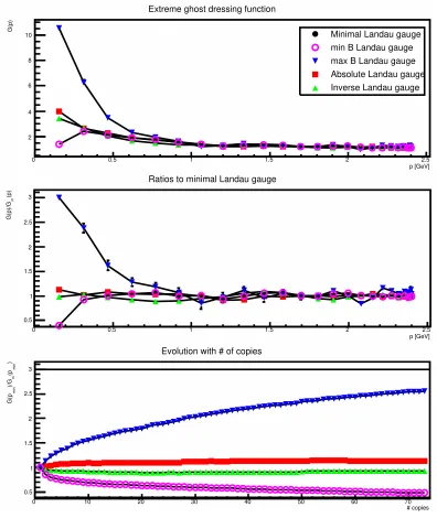
The situation is very different for the ghost. The impact strongly depends on the choice of gauge.
Choices, which utilize the quantityF show, however, also very little change, again in accordance
with previous investigations [4, 5, 9, 11, 20, 21, 23, 24, 26]. In this case also the dependence on the number of Gribov copies is mild. This drastically changes when studying gauges based on the
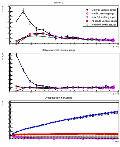
quantityb. Here, the impact is already at about half a GeV statistically significant. This is even
more pronounced in the case of the running coupling. This is not surprising, as the gluon propagator essentially does not change, and there is hence nothing to offset the squared effect from the ghost. This has also corresponding implications for the dependence on the number of included Gribov copies.
p [GeV]
0 0.5 1 1.5 2 2.5
]
-2
D(p) [GeV
0.5 1 1.5 2 2.5 3 3.5 4
Minimal Landau gauge min B Landau gauge max B Landau gauge Absolute Landau gauge Inverse Landau gauge Extreme gluon propagators
p [GeV]
0 0.5 1 1.5 2 2.5
(p)
m
D(p)/D
0.9 0.92 0.94 0.96 0.98 1 1.02 1.04 1.06 1.08 1.1
Ratios to minimal Landau gauge
# copies
0 10 20 30 40 50 60 70
(0)
m
D(0)/D
0.9 0.92 0.94 0.96 0.98 1 1.02 1.04 1.06 1.08 1.1 1.12
Evolution with # of copies
Figure 2.The gluon propagator for various gauges (top panel) and the ratio to its value in minimal Landau gauge (middle panel). The bottom panel shows the evolution of the ratio at zero momentum as a function of included
(genuine [30]) Gribov copies. Results are in three dimension with a lattice spacinga−1
=1.20 GeV and a volume
of (Na)3
=(48a)3
=(7.9 fm)3. Full lines in the bottom panel are from extrapolations in the number of Gribov
p [GeV]
0 0.5 1 1.5 2 2.5
G(p)
2 4 6 8
10 Minimal Landau gauge
min B Landau gauge max B Landau gauge Absolute Landau gauge Inverse Landau gauge Extreme ghost dressing function
p [GeV]
0 0.5 1 1.5 2 2.5
(p)
m
G(p)/G
0.5 1 1.5 2 2.5 3
Ratios to minimal Landau gauge
# copies
0 10 20 30 40 50 60 70
)
min
(p
m
)/G
min
G(p
0.5 1 1.5 2 2.5 3
Evolution with # of copies
Figure 3.The ghost dressing function for various gauges (top panel) and the ratio to its value in minimal Landau gauge (middle panel). The bottom panel shows the evolution of the ratio at the lowest possible momentum on this lattice, 157 MeV, as a function of included (genuine [30]) Gribov copies. Results are in three dimension with
a lattice spacinga−1
=1.20 GeV and a volume of (Na)3
=(48a)3
=(7.9 fm)3. Full lines in the bottom panel are
p [GeV]
0 0.5 1 1.5 2 2.5
[GeV]
α
0.2 0.4 0.6 0.8 1 1.2 1.4
Minimal Landau gauge min B Landau gauge max B Landau gauge Absolute Landau gauge Inverse Landau gauge
α
Extreme
p [GeV]
0 0.5 1 1.5 2 2.5
(p)
m
α
(p)/
α
1 2 3 4 5 6 7 8 9
Ratioto minimal Landau gauge
# copies
0 10 20 30 40 50 60 70
[GeV]
α
1 2 3 4 5 6 7 8 9
Evolution with # of copies
Figure 4.The ghost dressing function for various gauges (top panel) and the ratio to its value in minimal Landau gauge (middle panel). The bottom panel shows the evolution of the ratio at the lowest possible momentum on this lattice, 157 MeV, as a function of included (genuine [30]) Gribov copies. Results are in three dimension with
a lattice spacinga−1
=1.20 GeV and a volume of (Na)3
=(48a)3
=(7.9 fm)3. Full lines in the bottom panel are
4 Summary and the role of matter
The bottom line of this investigation is that some correlation functions, most notably the ghost propa-gator and quantities derived from it, depend strongly on the choice of gauge for momenta at or below roughly 500 MeV. However, this behavior is only quantitative in all cases studied. Furthermore, an
estimate of the precise size of this quantitative effect is obstructed by the quick rise in the number
of Gribov copies with volume. Nonetheless, this implies that a comparison of results from different
methods makes for some quantities only sense if the same gauge is chosen. Especially for the compar-ison of lattice and functional methods, this implies that still some effort needs to be invested to have full control over the implementation of the same gauge [4, 9, 15]. Still, expressions like (1) are already a step towards a continuum formulation, as they no longer make explicit reference to Gribov copies, but only to fields, and thus are easier to handle in continuum formulations. It is also encouraging that these formulations give the same result as the ones based on the individual manipulation of Gribov copies [11, 12].
A last issue concerns the influence of matter on the results presented here. The gauge conditions employed here, the (non-aligned [16]) Landau gauges are well-defined in the presence of any matter fields. However, they never include the matter fields explicitly. Especially, the presence of matter fields cannot turn a gauge copy in Landau gauge into something else or remove it from the gauge orbit. Thus, matter fields can at most give different residual gauge orbits different weights in the path integral.
While this subject has not yet been studied in great detail, it appears that matter in QCD-like situa-tions does not have any significant impact on this question [34, 35]. However, this drastically changes
when a Brout-Englert-Higgs effect is at work [34]: In marked contrast to the situation here, the
stan-dard algorithms do find no Gribov copies [34]. Whether this is an algorithmic deficiency or whether
indeed the residual gauge orbits in this case have a different number of Gribov copies is unclear. At
any rate, the corresponding implications are far reaching, and deserve a better understanding. This is especially true, as also continuum investigations support a change of behavior [36]. In this respect, studies of the superconformal case, as a third possibility, may also be useful, as also in this case a different behavior is motivated by continuum investigations [37, 38].
References
[1] R. Alkofer, L. von Smekal, Phys. Rept.353, 281 (2001), (2001),hep-ph/0007355
[2] C.S. Fischer, J. Phys.G32, R253 (2006), (2006),hep-ph/0605173
[3] D. Binosi, J. Papavassiliou, Phys. Rept.479, 1 (2009), (2009),0909.2536
[4] A. Maas, Phys. Rep.524, 203 (2013), (2013),1106.3942
[5] P. Boucaud et al., Few Body Syst.53, 387 (2012), (2012),1109.1936
[6] N. Vandersickel, D. Zwanziger, Phys.Rept.520, 175 (2012), (2012),1202.1491
[7] V.N. Gribov, Nucl. Phys.B139, 1 (1978), (1978)
[8] I.M. Singer, Commun. Math. Phys.60, 7 (1978), (1978)
[9] A. Maas, Phys. Lett.B689, 107 (2010), (2010),0907.5185
[10] A. Maas, PoSQCD-TNT-II, 028 (2011), (2011),1111.5457
[11] A. Maas, PoSConfinementX, 034 (2012), (2012),1301.2965
[12] A. Maas (unpublished), (unpublished)
[13] P. Hirschfeld, Nucl. Phys.B157, 37 (1979), (1979)
[14] L. von Smekal, M. Ghiotti, A.G. Williams, Phys. Rev.D78, 085016 (2008), (2008),0807.0480
[16] A. Maas, Mod. Phys. Lett.A27, 1250222 (2012), (2012)
[17] L. von Smekal, A. Jorkowski, D. Mehta, A. Sternbeck, PoSCONFINEMENT8, 048 (2008),
(2008),0812.2992
[18] C. Parrinello, G. Jona-Lasinio, Phys.Lett.B251, 175 (1990), (1990)
[19] J. Serreau, M. Tissier, A. Tresmontant, Phys.Rev.D89, 125019 (2014), (2014),1307.6019
[20] A. Cucchieri, Nucl. Phys.B508, 353 (1997), (1997),hep-lat/9705005
[21] V.G. Bornyakov, V.K. Mitrjushkin, Phys.Rev.D84, 094503 (2011), (2011),1011.4790
[22] S. Fachin, C. Parrinello, Phys.Rev.D44, 2558 (1991), (1991)
[23] A. Maas, Phys. Rev.D79, 014505 (2009), (2009),0808.3047
[24] P.J. Silva, O. Oliveira, Nucl. Phys.B690, 177 (2004), (2004),hep-lat/0403026
[25] M. Schaden, D. Zwanziger, Phys. Rev.D92, 025001 (2014), (2014),1412.4823
[26] A. Sternbeck, M. Müller-Preussker, Phys. Lett.B726, 396 (2012), (2012),1211.3057
[27] D. Zwanziger, Nucl. Phys.B412, 657 (1994), (1994)
[28] D. Henty, O. Oliveira, C. Parrinello, S. Ryan (UKQCD Collaboration), Phys.Rev.D54, 6923
(1996), (1996),hep-lat/9607014
[29] L. von Smekal, K. Maltman, A. Sternbeck, Phys. Lett.B681, 336 (2009), (2009),0903.1696
[30] A. Maas (2015), (2015),1510.08407
[31] A. Cucchieri, A. Maas, T. Mendes, Phys. Rev.D74, 014503 (2006), (2006),hep-lat/0605011
[32] M. Blank, A. Krassnigg, A. Maas, Phys. Rev.D83, 034020 (2011), (2011),1007.3901
[33] P. Costa, O. Oliveira, P.J. Silva, Phys.Lett.B695, 454 (2011), (2011),1011.5603
[34] A. Maas, Eur. Phys. J.C71, 1548 (2011), (2011),1007.0729
[35] A. Maas, JHEP1105, 077 (2011), (2011),1102.5023
[36] M. Capri, D. Dudal, M. Guimaraes, I. Justo, S. Sorella et al., Annals Phys.343, 72 (2013),
(2013),1309.1402
[37] M.A.L. Capri, M.S. Guimaraes, I.F. Justo, L.F. Palhares, S.P. Sorella, Phys. Lett.B735, 277
(2014), (2014),1404.7163