FULL PAPER
Magnetic field stretching at the top
of the shell of numerical dynamos
Diego Peña
1*, Hagay Amit
2and Katia J. Pinheiro
1,2Abstract
The process of magnetic field stretching transfers kinetic energy to magnetic energy and by that maintains dynamos against Ohmic dissipation. Stretching at the top of the outer core may play an important role at specific regions. High-latitude intense magnetic flux patches may be concentrated by flow convergence. Reversed flux patches may emerge due to expulsion of toroidal field advected to the core–mantle boundary by fluid upwelling. Here we analyze snapshots from self-consistent 3D numerical dynamos to unravel the nature of field–flow interactions that induces stretching secular variation at the top of the core. We find that stretching at the top of the shell has a significant influ-ence on the secular variation despite the relatively weak poloidal flow. In addition, locally stretching is often more effective than advection in particular at regions of significant field-aligned flow. Magnetic flux patches are concen-trated by fluid downwelling and dispersed by fluid upwelling. Stretching is more efficient than advection in intensify-ing magnetic flux patches. Both stretchintensify-ing and the poloidal flow mostly depend on the magnetic Prandtl number Pm. Decreasing Pm gives smaller poloidal flow but stronger stretching. Accounting for field–flow interactions in both the advection and stretching terms suggests that the magnetic Reynolds number overestimates the actual ratio of mag-netic advection to diffusion by ∼50 %. Morphological resemblance between local stretching in our dynamo models and local observed geomagnetic secular variation may suggest the presence of stretching at the top of the Earth’s core. Our results shed light on the kinematic origin of intense geomagnetic flux patches and may have implications to the convective state of the upper outer core.
© 2016 Peña et al. This article is distributed under the terms of the Creative Commons Attribution 4.0 International License (http://creativecommons.org/licenses/by/4.0/), which permits unrestricted use, distribution, and reproduction in any medium, provided you give appropriate credit to the original author(s) and the source, provide a link to the Creative Commons license, and indicate if changes were made.
Introduction
The geomagnetic field is generated by convective motions of an electrically conductive fluid in Earth’s rapidly rotat-ing liquid outer core. The field is measured by surface magnetic observatories and dedicated satellites. Geo-magnetic measurements are inverted for spherical har-monic models which can be downward continued to the top of the region of field generation, i.e., the core–mantle boundary (CMB). Temporal changes in the geomagnetic field termed secular variation (SV) provide vital insight into the fluid dynamics and dynamo action at the top of the core. Indeed, geomagnetic field and SV models (e.g., Jackson et al. 2000; Olsen and Mandea 2008) have been used as constraints on numerical dynamo simulations (e.g., Christensen et al. 1998, 2010; Aubert et al. 2013)
or to infer various aspects of Earth’s core dynamics (e.g., Finlay and Jackson 2003), in particular the fluid flow just below the CMB (for a review, see Holme 2007).
According to dynamo theory, the SV is comprised of magnetic advection, stretching and diffusion. Mag-netic field advection transfers magMag-netic energy from one degree to another, whereas magnetic field stretch-ing transfers kinetic energy to magnetic energy and by that maintains dynamos against Ohmic dissipation (e.g., Moffatt 1978; Mininni 2011). Therefore, magnetic field stretching is responsible for dynamo action. Better understanding of the field–flow interactions that yield magnetic field stretching is therefore fundamental for dynamo theory. Of course dynamo action might not nec-essarily occur at the entire outer core. For example, the dynamo may be deep seated due to stable stratification at the top of core, as was argued for Mercury (Christensen 2006) and for the Earth (Pozzo et al. 2012; Gubbins and Davies 2013). Here, however, we focus on the CMB,
Open Access
*Correspondence: [email protected]
1 Geophysics Department, Observatório Nacional, CEP: 20921-400 Rio de Janeiro, Brazil
for comparison with geomagnetic field and SV models inferred from observations.
Fluid dynamics systems are often characterized by non-dimensional numbers. These numbers give valu-able physical intuition concerning the relative impor-tance of different processes in the system, for example the dominant force acting on the fluid and the role of turbulence. However, calculations of dynamo-related non-dimensional numbers using typical scales and ignoring field–flow interactions might provide non-representative values. Finlay and Amit (2011) calculated various alternative magnetic Reynolds numbers Rm that took into account different length scales of core dynam-ics. They extrapolated SV spectra to obtain an advective length scale; inferences from numerical dynamos (Amit and Christensen 2008) and from expansion of reversed flux patches (Chulliat and Olsen 2010) were used to infer a diffusive length scale. Finlay and Amit (2011) focused on magnetic field advection and ignored mag-netic field stretching. It is important to re-evaluate non-dimensional numbers in order to better understand core dynamics in light of field–flow interactions and account-ing for magnetic stretchaccount-ing effects.
Global criteria for characterizing the observed geo-magnetic field (Christensen et al. 2010) are practical because the field spectrum is decreasing with degree (most energy at largest scale, i.e., dipole). In contrast, the geomagnetic SV spectrum is increasing with degree, which is a problem for global characterization. Some SV features like westward drift (Finlay and Jackson 2003) or Pacific/Atlantic dichotomy (Christensen and Olson 2003) could be related to external forcings such as gravitational coupling between the inner core and the mantle (Aubert et al. 2013) or core–mantle thermal interactions (Holme et al. 2011) rather than core convection itself. Alterna-tively, geomagnetic SV may be locally studied. Robust geomagnetic field features such as intense normal and reversed flux patches have a particular signature on the SV. Local analysis of field–flow interactions may provide a detailed interpretation of the SV in the vicinity of these robust field features.
Stretching may play an important role in specific regions of the CMB, such as high-latitude intense geo-magnetic flux patches. These robust non-axisymmetric features typically reside near the edge of the inner core tangent cylinder (Jackson et al. 2000), possibly due to flow convergence at these latitudes (Olson et al. 1999). In rapidly rotating numerical dynamo models surface con-vergence is correlated with columnar cyclones (Olson et al. 2002; Amit et al. 2007), so the flow near these patches has a large field-aligned component and pro-duces little magnetic advection (Finlay and Amit 2011). Regardless of whether the locations of downwellings are
directly related to a thermal mantle anomaly (Gubbins 2003) or to the chaotic time-dependent buoyancy at the top of the core, the kinematic relation between concen-trated magnetic flux and fluid downwelling is expected from the stretching term in the radial magnetic induction equation.
Magnetic field stretching may also be the underlying mechanism for regions of weak field intensity at Earth’s surface. Striking deviations of the geomagnetic field from axial dipolarity appear in the form of reversed flux patches, i.e., regions on the CMB where the sign of the radial field is opposite to that of the axial dipole field. In the past century, the most intense and extensive reversed flux patches have been growing and intensifying at the southern Atlantic of the CMB (e.g., Jackson et al. 2000; Olsen et al. 2014). At Earth’s surface these structures are expressed as a notably low-intensity zone termed the South Atlantic Magnetic Anomaly (Hartmann and Pacca 2009). The field intensity at this region is at present decreasing at rates of up to 12 % over the past 30 years (Finlay et al. 2010), much faster than the decline of the geomagnetic dipole moment (Olson and Amit 2006; Fin-lay 2008). It has been proposed that reversed flux patches emerge due to expulsion of toroidal field (Bloxham 1986) which is transported to the CMB by fluid upwelling (e.g., Aubert et al. 2008a).
It is under debate whether any stretching effects pre-vail at the top of Earth’s core. Seismic studies (Helffrich and Kaneshima 2010) and revised estimates of large core thermal conductivity from mineral physics calculations (Pozzo et al. 2012; Koker et al. 2012) suggest that the top of the core is stably stratified (Gubbins and Davies 2013). This may indicate that the flow just below the CMB is purely toroidal and no stretching SV is present there, although the radial flow may penetrate a stably stratified layer, e.g., if the convection columns are large enough (Takehiro and Lister 2001) or in the presence of certain waves (Buffett 2014). Low geomagnetic SV at special points where the radial field gradient is zero also supports stable stratification (Whaler 1980), but uncer-tainty in their exact locations renders such an interpreta-tion quesinterpreta-tionable (Whaler and Holme 2007). In contrast, Zhang et al. (2015) claimed that the thermal conductivity is as low as previously estimated and thus the whole of the outer core convects. Regional interpretations of the geomagnetic SV also favor some local upwelling/down-welling (Olson and Aurnou 1999; Chulliat et al. 2010; Amit 2014).
models rely on poloidal flow to project CMB flows to the volume of the core (Pais and Jault 2008; Gillet et al. 2009). Lesur et al. (2015) inverted geomagnetic data simultane-ously for the field and the core flow. When a purely toroi-dal flow was incorporated in the inversion the data could not be adequately fitted, in contradiction to upper core stratification. However, inclusion of weak poloidal flow was sufficient to explain the SV. Lesur et al. (2015) con-cluded that the upper core is weakly stratified.
In this paper, we analyze output from self-consistent 3D numerical dynamos to unravel the nature of field– flow interactions and the contribution of magnetic field stretching to the SV at the top of the spherical shell. Ana-lytical and statistical tools are designed to quantify these kinematic processes. We zoom-in to specific regions on the outer boundary to explore the kinematic origins of intense normal and reversed magnetic flux patches. The dependence of the results on the dynamo control param-eters is explored. The results are discussed in the context of geomagnetic field and SV models.
Methods
Numerical dynamo models
Fluid motions in Earth’s outer core are governed by the magnetohydrodynamics equations: Navier–Stokes, mag-netic induction, conservation of energy and mass (con-tinuity for an incompressible fluid). In non-dimensional form these equations can be written (e.g., Olson et al. 1999) as follows:
where u is the fluid velocity, B is the magnetic field, T is temperature (or more generally co-density), t is time, zˆ
is a unit vector in the direction of the rotation axis, P is pressure, r is the position vector, ro is the core radius, and
ǫ is heat (or buoyancy) source or sink. The magnetic field changes in time [first term in (2)] due to its generation by the fluid flow [second term in (2)] and its destruction (or (1)
magnetic diffusion) due to the finite electrical conductiv-ity of the outer core fluid [third term in (2)]. In return the flow varies in time [first term in (1)] due to all the forces acting on it, including the magnetic Lorentz force [last term in (1)].
Four non-dimensional parameters in (1)–(3) con-trol the dynamo action. The heat flux Rayleigh number (Olson and Christensen 2002) represents the strength of buoyancy force driving the convection relative to retard-ing forces
where α is thermal expansivity, go is gravitational
accel-eration on the outer boundary at radius ro, qo is the mean
heat flux across the outer boundary, D is shell thickness,
k is thermal conductivity, κ is thermal diffusivity, and ν is
kinematic viscosity. The Ekman number represents the ratio of viscous and Coriolis forces
where Ω is the rotation rate. The Prandtl number is the
ratio of kinematic viscosity to thermal diffusivity
and the magnetic Prandtl number is the ratio of kine-matic viscosity to magnetic diffusivity
The condition for dynamo action is that the magnetic field generation term will sufficiently exceed the diffusion term in (2). The scaled ratio between these two terms is given by the magnetic Reynolds number
where U is a typical velocity scale.
Numerical dynamos provide self-consistent solutions to the full set of Eqs. (1)–(5) in a spherical shell (Chris-tensen and Wicht 2007). We used the numerical imple-mentation MagIC (Wicht 2002). Due to computational limitations, dynamo simulations use control parameters very far from Earth-like conditions, and therefore, relat-ing the results to the real core conditions is challengrelat-ing. Our chosen control parameters (Table 1) are even more moderate than what modern computers are capable of. The reason is that smaller E values produce such small-scale structures that the local relations between the field and the flow would become difficult to interpret. We
focus on dynamos in the non-reversing dipole-domi-nated regime (e.g., Kutzner and Christensen 2002; Chris-tensen and Aubert 2006).
The shell geometry is identical to Earth’s core with an inner to outer boundary radii ratio of 0.35. The inner and outer boundaries of the shell are set to be insulating and rigid. To simulate generic thermochemical convec-tion (e.g., Aubert et al. 2008b), on the inner core bound-ary fixed co-density is set, on the outer boundbound-ary fixed heat flux is prescribed, and the source/sink term in (3) is set to ǫ =0. The number of radial grid points Nr is
chosen to accommodate at least five grid points across the Ekman boundary layer. In our models, Nr varies
from 49 for the larger E=1×10⁻³ cases to 61 for the
lower E =1×10⁻⁴ cases. Horizontal resolution is also increased with decreasing Ekman number, from maxi-mum degree and order ℓmax=64 for the E=1×10⁻³
cases to ℓmax =96 for the E=1×10⁻⁴ cases.
It is of particular interest to examine the radial com-ponent of the induction equation just below the outer boundary, because only the radial component of the geo-magnetic field at the CMB is accessible from observa-tions. The radial component of (2) at the top of the shell where the radial velocity vanishes is
where Br is the radial field, uh is the 2D velocity vector
tangent to the spherical surface, ∇h= ∇ − ∂
∂r, and r
is the radial coordinate. The first term in (11) is the SV, the second term represents magnetic field advection, the third term represents magnetic field stretching, and the term on the right-hand side denotes magnetic diffusion.
(11)
The frozen-flux theory (Roberts and Scott 1965) assumes that the majority of SV on short timescales and large length scales is produced by the advection and stretching action due to the velocity field rather than dif-fusion of the magnetic field. Based on the observed SV and inferences from mineral physics experiments Rm
∼ 500 in Earth’s outer core (e.g., Bloxham and Jackson
1991), supporting the frozen-flux hypothesis. Under this assumption (11) simplifies to
This equation is the common starting point for mod-eling the flow at the core surface (e.g., Holme 2007). It is termed the frozen-flux induction equation, because accordingly magnetic field lines are simply carried by the flow.
The radial magnetic field Br and the tangential velocity
uh were taken at the top of the free stream (just below the
Ekman boundary layer) to analyze the different terms of the radial induction equation. Note that in the dynamo models at the top of the free stream the radial velocity is more than an order of magnitude smaller than the tan-gential velocity hence (11) holds. In order to obtain sta-tistics of the dynamical characteristics of the simulations, for each dynamo model ten snapshots were taken at arbi-trary times enough separated so that their structures are non-correlated. Overall, 90 snapshots were globally ana-lyzed, of which more than 350 zoom-ins to local regions of intense magnetic flux patches were selected.
Statistical measures
We calculate several statistical properties to analyze the results, including global and local RMS ratios (X/Y) Table 1 Dynamo models control parameters
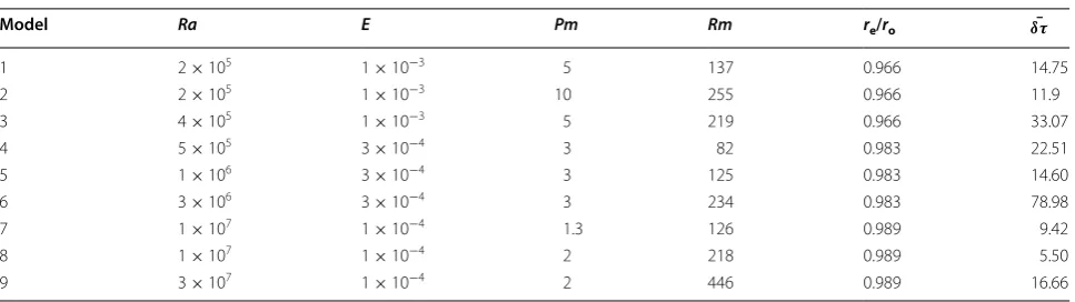
The Rayleigh number is Ra, the Ekman number is E and the magnetic Prandtl number is Pm. For all models we set the Prandtl number as Pr=1. The magnetic Reynolds number Rm is calculated based on the total kinetic energy in the shell, re denotes the radial level at which the simulations were analyzed, and δτ¯ denotes the average time difference between successive snapshots in units of magnetic advection time
spherical surface at the top of the free stream. We com-pute the ratio of RMS stretching to RMS advection St/Ad as well as the ratio of RMS poloidal flow to RMS toroi-dal flow P/T. We also calculate the spatial correlation
coefficient between tangential divergence δh≡ ∇h· �uh
and plus/minus radial vorticity ωr ≡ ˆr·∇ × �u (where rˆ is
the radial unit vector) in the Northern/Southern Hemi-sphere, respectively, termed helical flow by Amit and Olson (2004)
where θ is co-latitude. The correlation coefficient between the absolute radial field and downwelling is corr(|Br|,δ−h)
with δ−h defined by
Likewise, the correlation coefficient between absolute radial field and upwelling is corr(|Br|,δ+h) with δ+h defined by
Local analyses are classified by polarity, i.e., normal or reversed, and by latitude. High latitudes are arbitrar-ily defined by patches that are centered at higher than 45° latitude. Classified this way, four types of patches are possible: normal polarity at high latitudes (HN), normal polarity at low latitudes (LN), reversed polarity at high latitudes (HR) and reversed polarity at low latitudes (LR). In addition, normalized integrated values allow evalua-tion of level of cancellaevalua-tion in a given region
where f is the studied quantity in a region S and dS =r2sinθdφdθ is a spherical surface increment. If all advection has the same sign in a region then ξa=1 , whereas if the advection has alternating signs of equal amount then ξa=0. The same type of interpretation holds for the stretching efficiency ξs. In order to test
whether the stretching intensifies or weakens the mag-netic flux, the normalized integrated value of their prod-uct is evaluated:
If the stretching SV and Br have the same sign (i.e., field intensification by stretching) then ξe>0, whereas if
(13)
Next we estimate an effective magnetic Reynolds num-ber that accounts for field–flow interactions. For the advective part, following Finlay and Amit (2011) we cal-culate the angle γ between the vectors uh and ∇hBr so that (π/2−γ ) is the angle between a Br-contour and the core surface flow uh. The level of field-aligned flow is
rep-resented by
If the field and the flow are perfectly aligned then
γ =π/2 and advection is zero, whereas if the flow is perpendicular to Br-contours then γ =0 and advection efficiency is optimal. Accordingly, the effective advective magnetic Reynolds number Rma is then
The effective stretching magnetic Reynolds number Rms
is simply
In order to combine Rma and Rms the correlation
between the two SV contributions should be accounted for. We therefore compute the interaction between the two terms by
If St and Ad are correlated then ξRm=1. If St and Ad
are non-correlated then ξRm= √
1+c2/(1+c) where
c is their amplitude ratio. In this case a minimum of
ξRm= √
2/2 is obtained for c=1 (i.e., equal advection and stretching amplitudes). Finally, if St and Ad are anti-correlated then ξRm= | −1+c|/(1+c). In this case for c=1ξRm=0, i.e., advection and stretching cancel each
other to yield zero inductive SV. The effective magnetic Reynolds number is then given by
To get some intuition to the quantities cosγ and ξRm we
report their values for some large-scale synthetic cases. For the radial field, we use a dipole with present-day Earth-like tilt (Olsen et al. 2014) and for the flow we use large-scale degree-1 toroidal and poloidal flows (Table 2). Obviously for the toroidal flows stretching is zero and
ξRm=1. Because the dipole field is dominantly axial,
the most effective advection scenario (i.e., largest cosγ)
occurs when the flow is oriented north-south (P0 1). Over-all the two quantities cosγ and ξRm are clearly distinctive
with either one larger for different cases.
Finally, we examine the dependence of the statistical quantities on the non-dimensional control parameters of the dynamo models. Each quantity (St/Ad, P/T, Hu, etc.)
may be expressed as a generic power law:
where f is the statistical quantity and C, a, b, c are fit-ting coefficients. The relative misfit σr of the power law is given by
where fdyn is the statistical quantity obtained from the
dynamo models and n is the number of dynamo models analyzed. Relative misfits larger than an arbitrary thresh-old value of 0.07 were considered inadequate, and in these cases, the fits were not interpreted.
The power law fits (23) obtained by the misfit minimi-zation (24) are applied to time-average statistical quanti-ties. The time-dependence is expressed by the standard deviation (Tables 3, 4). Note that the standard deviation was not used to assess the fits.
This paper contains many variables. While some are conventional, others were introduced to denote newly defined properties. For clarity we list in the “Appendix” all the variables used in this paper.
Results
Kinematics of intense magnetic flux patches
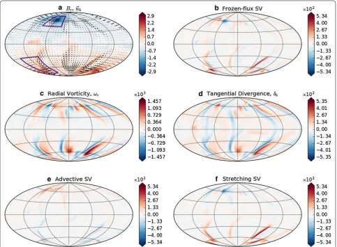
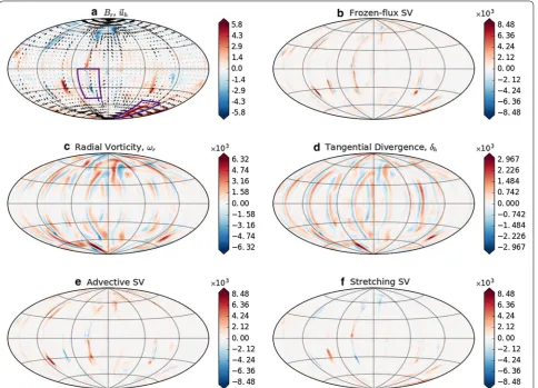
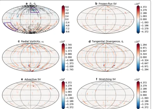
Figure 1 shows an arbitrary snapshot from dynamo model 4. As in all models considered in this study, the radial magnetic field on the outer boundary exhibits axial dipole dominance (Fig. 1a). The tangential diver-gence δh is highly correlated with the radial vorticity ωr in the Southern Hemisphere and highly anti-correlated in the Northern Hemisphere (Fig. 1c, d). The toroidal flow dominates over the poloidal flow at the top of the free stream (P/T <1). Nevertheless globally, the stretching (23)
contribution to the frozen-flux SV is larger than that of advection (Fig. 1e, f). Intense magnetic flux patches pre-sent positive and negative correlations with downwelling and upwelling structures, respectively. Because our dynamo models are dominated by the axial dipole, most of the intense flux patches are obviously of normal polar-ity at high latitudes (HN) and only a few are normal (LN) and reversed (LR) at low latitudes. The flux patches are rather large scale and are significantly more intense than their surroundings.
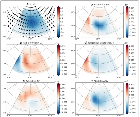
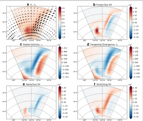
Figure 2 shows a typical intense high-latitude normal polarity (HN) magnetic flux patch (see upper polygon in Fig. 1a). This patch is located close to the center of an anti-clockwise vortex (Fig. 2a, c) that is highly corre-lated with a downwelling structure (Fig. 2d). The flow in this region is predominately toroidal. The main part of the flow is aligned with the Br-contours (Fig. 2a), caus-ing non-efficient advection (Fig. 2e). In contrast, the high correlation between the magnetic flux patch and the downwelling structure produces a strong stretching SV (Fig. 2f) that locally intensifies the magnetic field with an efficiency of ξe=0.94. Consequently, the local stretching SV is remarkably twice larger than advective SV.
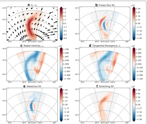
Another HN (lower polygon in Fig. 1a) is located west of a strong southward flow (Fig. 3a). This flow system produces an intense advective SV at the eastern part of the patch. In the western part, the flow and hence the advection are weak. Despite the relatively weak poloidal flow, the downwelling structure shown in Fig. 3d pro-duces intense stretching SV (Fig. 3f). In this patch, the stretching SV is only slightly larger than advective SV, but it is still able to locally intensify the magnetic field with an efficiency of ξe=0.87.
Overall we found three types of intense magnetic flux patches (out of the four possible types): Most of them are high-latitude normal polarity flux patches (HN), whereas a smaller number are low-latitude normal polarity (LN) and low-latitude reversed polarity (LR). Reversed flux patches at high latitudes (RH) are rare. The same holds for all the dynamo models examined here. From hereafter we therefore report local analyses of HN, LN and LR only.
Next we examine a dynamo model with a larger Ra, and otherwise all parameters unchanged (Table 1). Figure 4 shows an arbitrary snapshot from dynamo model 6. As in model 4, the radial magnetic field has the characteristic axial dipolar dominance and the flow is predominantly toroidal. The global correlation of radial vorticity and tangential divergence is again high. Intense magnetic flux patches are positively correlated with downwelling struc-tures and negatively with upwelling strucstruc-tures. However, the field and flow features are smaller scale and advection is globally stronger than stretching.
Table 2 Field–flow interferences in synthetic cases
Table 3 Global statistics
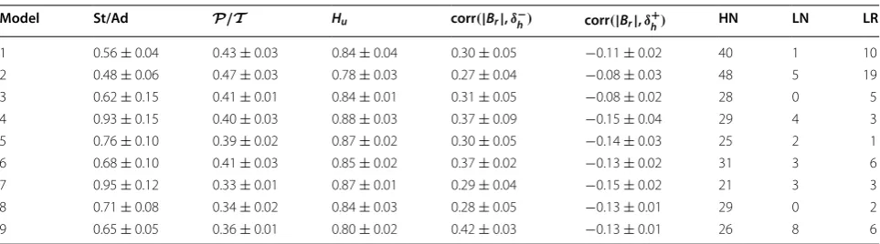
Dynamo models time-average and standard deviation values. St/Ad is stretching/advection RMS ratio, and P/T is poloidal/toroidal flow RMS ratio. Hu is the helical flow correlation (13), corr(|Br|,δ−h) and corr(|Br|,δ+h) are the correlations between the absolute radial magnetic field and downwelling (14) and upwelling (15),
respectively. Also, the number of analyzed magnetic flux patches of each type is given: high-latitude normal intense flux patches (HN), low-latitude normal intense flux patches (LN) and low-latitude reversed flux patches (LR)
Model St/Ad P/T Hu corr(|Br|,δh−) corr(|Br|,δh+) HN LN LR
1 0.56 ± 0.04 0.43 ± 0.03 0.84 ± 0.04 0.30 ± 0.05 −0.11 ± 0.02 40 1 10 2 0.48 ± 0.06 0.47 ± 0.03 0.78 ± 0.03 0.27 ± 0.04 −0.08 ± 0.03 48 5 19 3 0.62 ± 0.15 0.41 ± 0.01 0.84 ± 0.01 0.31 ± 0.05 −0.08 ± 0.02 28 0 5 4 0.93 ± 0.15 0.40 ± 0.03 0.88 ± 0.03 0.37 ± 0.09 −0.15 ± 0.04 29 4 3 5 0.76 ± 0.10 0.39 ± 0.02 0.87 ± 0.02 0.30 ± 0.05 −0.14 ± 0.03 25 2 1 6 0.68 ± 0.10 0.41 ± 0.03 0.85 ± 0.02 0.37 ± 0.02 −0.13 ± 0.02 31 3 6 7 0.95 ± 0.12 0.33 ± 0.01 0.87 ± 0.01 0.29 ± 0.04 −0.15 ± 0.02 21 3 3 8 0.71 ± 0.08 0.34 ± 0.02 0.84 ± 0.03 0.28 ± 0.05 −0.13 ± 0.01 29 0 2 9 0.65 ± 0.05 0.36 ± 0.01 0.80 ± 0.02 0.42 ± 0.03 −0.13 ± 0.01 26 8 6
Table 4 Local statistics
Dynamo models time-average and standard deviation values for each patch type. RMS ratios, correlations and patch types are the same as in Table 3. ξa and ξs are the absolute normalized integrated values of advection and stretching SV, respectively, ξe is the normalized integrated value of the product of stretching SV and Br. x¯ denotes averages over all dynamo models
Model Patch type St/Ad P/T Hu corr(|Br|,δh−) corr(|Br|,δh+) ξa ξs ξe
1 HN 0.69 ± 0.23 0.34 ± 0.05 0.91 ± 0.11 0.44 ± 0.19 −0.28 ± 0.08 0.44 ± 0.09 0.76 ± 0.09 0.92 ± 0.09 LN 0.28 ± 0.00 0.60 ± 0.00 0.70 ± 0.00 0.38 ± 0.00 −0.34 ± 0.00 0.11 ± 0.00 0.31 ± 0.00 0.62 ± 0.00 LR 0.48 ± 0.14 0.63 ± 0.11 0.79 ± 0.19 0.42 ± 0.17 −0.18 ± 0.13 0.07 ± 0.04 0.20 ± 0.06 0.68 ± 0.13 2 HN 0.55 ± 0.21 0.40 ± 0.07 0.83 ± 0.09 0.29 ± 0.19 −0.19 ± 0.09 0.28 ± 0.09 0.59 ± 0.18 0.77 ± 0.20 LN 0.33 ± 0.10 0.59 ± 0.12 0.71 ± 0.23 0.43 ± 0.24 −0.17 ± 0.13 0.11 ± 0.06 0.38 ± 0.16 0.56 ± 0.22 LR 0.43 ± 0.16 0.79 ± 0.14 0.59 ± 0.22 0.28 ± 0.22 −0.04 ± 0.19 0.11 ± 0.08 0.25 ± 0.13 0.62 ± 0.19 3 HN 0.60 ± 0.19 0.33 ± 0.05 0.91 ± 0.03 0.30 ± 0.18 −0.19 ± 0.11 0.24 ± 0.08 0.56 ± 0.16 0.87 ± 0.06
LN – – – – – – – –
LR 0.65 ± 0.27 0.61 ± 0.06 0.82 ± 0.09 0.60 ± 0.14 −0.20 ± 0.03 0.26 ± 0.08 0.52 ± 0.13 0.84 ± 0.09 4 HN 1.27 ± 0.51 0.32 ± 0.07 0.87 ± 0.20 0.71 ± 0.10 −0.39 ± 0.11 0.63 ± 0.13 0.61 ± 0.13 0.85 ± 0.09 LN 1.10 ± 0.29 0.39 ± ± 0.02 0.91 ± 0.05 0.78 ± 0.03 −0.48 ± 0.08 0.58 ± 0.14 0.35 ± 0.09 0.57 ± 0.11 LR 0.24 ± 0.01 0.69 ± 0.01 0.52 ± 0.06 −0.23 ± 0.06 0.14 ± 0.01 0.06 ± 0.00 0.28 ± 0.02 0.24 ± 0.01 5 HN 0.95 ± 0.30 0.32 ± 0.05 0.83 ± 0.14 0.54 ± 0.13 −0.35 ± 0.06 0.57 ± 0.14 0.75 ± 0.08 0.93 ± 0.04 LN 0.43 ± 0.00 0.42 ± 0.00 0.91 ± 0.00 0.57 ± 0.00 −0.22 ± 0.00 0.47 ± 0.00 0.72 ± 0.00 0.94 ± 0.00 LR 0.72 ± 0.00 0.86 ± 0.00 0.71 ± 0.00 0.49 ± 0.00 −0.23 ± 0.00 0.09 ± 0.00 0.16 ± 0.00 0.67 ± 0.00 6 HN 0.74 ± 0.15 0.34 ± 0.05 0.91 ± 0.04 0.40 ± 0.18 −0.27 ± 0.10 0.39 ± 0.07 0.69 ± 0.11 0.87 ± 0.10 LN 0.69 ± 0.15 0.60 ± 0.07 0.91 ± 0.01 0.54 ± 0.18 −0.18 ± 0.00 0.12 ± 0.10 0.32 ± 0.26 0.82 ± 0.04 LR 0.68 ± 0.13 0.73 ± 0.31 0.85 ± 0.06 0.54 ± 0.18 −0.19 ± 0.03 0.11 ± 0.06 0.17 ± 0.08 0.76 ± 0.09 7 HN 1.18 ± 0.28 0.28 ± 0.08 0.80 ± 0.15 0.54 ± 0.13 −0.30 ± 0.07 0.59 ± 0.09 0.62 ± 0.08 0.89 ± 0.06 LN 0.81 ± 0.20 0.40 ± 0.01 0.91 ± 0.02 0.54 ± 0.16 −0.25 ± 0.12 0.55 ± 0.06 0.51 ± 0.05 0.74 ± 0.04 LR 1.12 ± 0.12 0.58 ± 0.01 0.81 ± 0.04 0.48 ± 0.06 −0.09 ± 0.02 0.08 ± 0.06 0.04 ± 0.04 0.67 ± 0.05 8 HN 0.78 ± 0.20 0.27 ± 0.04 0.83 ± 0.12 0.45 ± 0.15 −0.30 ± 0.06 0.50 ± 0.12 0.68 ± 0.08 0.89 ± 0.06
LN – – – – – – – –
LR 0.93 ± 0.00 0.94 ± 0.00 0.60 ± 0.00 0.57 ± 0.00 −0.18 ± 0.00 0.14 ± 0.00 0.20 ± 0.00 0.63 ± 0.00 9 HN 0.68 ± 0.15 0.31 ± 0.06 0.81 ± 0.11 0.48 ± 0.18 −0.24 ± 0.07 0.32 ± 0.06 0.63 ± 0.07 0.84 ± 0.04 LN 0.61 ± 0.13 0.45 ± 0.07 0.82 ± 0.04 0.51 ± 0.05 −0.23 ± 0.04 0.28 ± 0.05 0.54 ± 0.07 0.83 ± 0.02 LR 0.85 ± 0.09 0.67 ± 0.17 0.70 ± 0.06 0.55 ± 0.19 −0.22 ± 0.07 0.20 ± 0.20 0.25 ± 0.25 0.88 ± 0.07 ¯
x HN 0.82 0.32 0.86 0.46 −0.28 0.44 0.65 0.90
LN 0.61 0.49 0.84 0.53 −0.27 0.32 0.45 0.73
Figure 5 shows an intense high-latitude normal polar-ity flux patch (lower polygon in Fig. 4a). This HN is at the center of a clockwise vortex correlated with a down-welling structure (Fig. 5c, d). A large part of the flow is field aligned, so advection is confined to a region close to the patch center (Fig. 5a, e). The interaction of the downwelling structure with the intense flux patch on the northern part produces a strong stretching struc-ture (Fig. 5f), but some shift in the southern part leads to moderate St/Ad RMS ratio. The stretching and advective contributions to the SV are comparable despite the rela-tively weak poloidal flow.
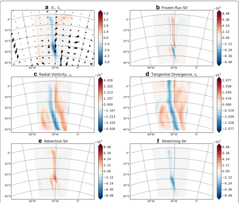
Next we analyze an LR (upper polygon in Fig. 4a). The southward flow is roughly perpendicular to the Br -con-tours (Fig. 6a), producing a strong advective SV (Fig. 6e). The downwelling structure in Fig. 6d is well correlated with this reversed flux patch, and hence the stretching
structure shown in Fig. 6f also presents an important contribution to the SV. In contrast, stretching locally intensifies the magnetic field with a smaller efficiency than in the HN (Fig. 5). In addition, the poloidal flow is relatively larger than in HN.
Dynamo model 9 (Fig. 7) has lower E and larger Ra
resulting in larger Rm (Table 1) and a more complex behavior. As in previous models, the flow is predomi-nately toroidal and tangential divergence and radial vor-ticity correlation is high. However, the magnetic flux patches in this model are small scale and a larger number of them appear at low latitudes (Table 3). The main con-tribution to the SV is advective.
Figure 8 shows an HN (upper polygon in Fig. 7a) from dynamo model 9. This patch is at the center of an anti-clockwise vortex (Fig. 8a) related to a downwelling structure (Fig. 8d). Advection is effective at the peak
Fig. 1 Snapshot from dynamo model 4: a radial magnetic field Br (in colors) and the tangential flow uh (black arrows). The upper and lower polygons denote the zoom-in zones shown in Figs. 2 and 3, respectively. b The frozen-flux SV, c radial vorticity ωr, d tangential divergence δh, e advective SV and f stretching SV. All plots are at a radial level just below the Ekman boundary layer (re in Table 1). All variables are non-dimensional. The global
of the patch (see Fig. 8e). In contrast, the downwelling structure exhibits a phase shift with the Br patch result-ing in a weak stretchresult-ing (Fig. 8f) and thus an advective dominant SV.
In dynamo model 9 some intense normal polarity flux patches appear at low latitudes (LN). Figure 9 shows an LN (lower polygon in Fig. 7a). This patch is located west of an anti-clockwise vortex correlated with an upwelling structure (Fig. 9d). A large component of the flow is perpendicular to the Br-contours and consequently, the advective SV efficiency is high. Stretching is less efficient due to the phase shift between the downwelling structure (Fig. 9d) and the intense flux patch. In this low-latitude
intense flux patch, the stretching locally intensifies the magnetic field with an efficiency of ξe=0.88.
Table 3 summarizes the global statistics of all snap-shots from each dynamo simulation, while Table 4 sum-marizes the local statistics per patch type. In all models, both globally and for the patches, absolute magnetic flux is positively/negatively correlated with downwelling/ upwelling, respectively. The best global correlation of absolute magnetic flux and downwelling is obtained in dynamo model 9 (Table 3). In dynamo model 4 for HN and LN the flux to downwelling correlations are highest, while LR has the best flux to downwelling correlation in dynamo model 3 (Table 4).
a
c
e
d
f
b
Fig. 2 Intense high-latitude normal polarity magnetic flux patch (HN) in dynamo model 4 (upper polygon in Fig. 1a). a Radial magnetic field Br (in colors) and tangential velocity uh (black arrows), b frozen-flux secular variation SV, c radial vorticity ωr, d tangential divergence δh, e advective SV and
f stretching SV. The local statistics for this patch are: St/Ad=2.01; P/T =0.23; Hu=0.97; corr(|Br|,δh−)=0.71; corr(|Br|,δh+)= −0.36; ξa=0.66;
Parameters dependence
In order to examine more quantitatively the dependence of the statistical measures on the non-dimensional con-trol parameters, we used a generic power law (23). The fitting parameters C, a, b and c were calculated using a conventional least-squared fit. Power law fits were applied for global and local measures.
The best fit for the global St/Ad ratio is given by
with a relative misfit of σr =0.063. In (25) the E and Ra powers are comparable, which motivates the following approximation:
(25) St/Ad=3.245·E−0.183·Ra−0.174·Pm−0.469
(26) St/Ad≈C·(E·Ra)a·Pmc
The best fit of (26) is
with σr=0.063. Then (27) could be approximated in log-arithmic scale as
Figure 10a confirms the similarity between the −0.152
slope of the fitted linear curve and the approximated power of −1
6 in (28). The parameter dependence of the
global St/Ad is thus given by
(27)
St/Ad≈3.508(E·Ra)−0.172·Pm−0.482
(28) log(St/Ad)≈logC−1
6log(E Ra Pm 3)
(29)
St/Ad≈2.996(E Ra Pm3)−16
a
c
e
f
b
d
Considering the modified Rayleigh number Ra′= E·RaPr
(e.g., Olson et al. 1999), and Pr=1, Eq. (29) could be written as
Globally, relative stretching in the dynamo models increases with increasing rotation (decreasing E), but decreases when convection (Ra) and electrical conduc-tivity (Pm) increase. The dependence is strongest on Pm
(30).
We followed a similar fitting process for the St/Ad ratio of HN. The parameter dependence of St/Ad of HN is given by (Fig. 10b)
In qualitative agreement with the global case (Fig. 10a), relative stretching increases with rotation, but decreases (30)
St/Ad≈2.996(Ra′Pm3)−16
(31)
St/Ad≈10.489(Ra′Pm2)−13
when convection and electrical conductivity increase. In high-latitude normal intense flux patches (HN), relative stretching exhibits a strong dependence on Pm, but less than in global.
We also attempted to find power law fits for St/Ad of LN and LR, but no satisfactory fit (large σr) was found. The same holds for the other statistical quantities. Fits were therefore obtained for global and HN but not for LN and LR.
Next we fitted the global P/T ratio. The best fit is
with σr =0.021. The Pm power is dominant, motivating
with σr =0.022. Then (33) may be approximated in loga-rithmic scale as
(32)
P/T =0.373·E−0.002·Ra−0.008·Pm0.153
(33) P/T ≈0.321Pm0.175
(34)
log(P/T)≈logC+1
6log(Pm)
The 0.179 slope in Fig. 11a well approximates the −16
pre-diction in (34). Then, the parameter dependence of global
P/T is approximated by
Globally, the relative poloidal flow is mostly influenced by
Pm, increasing with increasing electrical conductivity. We followed similar fitting process for the P/T ratio of
HN. The parameter dependence of P/T in HN is given
by (Fig. 11b)
(35) P/T ≈0.319Pm16
(36) P/T ≈0.261Pm16
In HN, the relative poloidal flow also increases when electrical conductivity increases.
We also attempted to fit the global and local Hu ratio.
In both cases, we found much lower powers than in (30), (31), (35) and (36), indicating that the parameter depend-ence of Hu is weak. We therefore do not plot this
param-eter dependence.
The St/Ad ratio is a good measure of the stretching influence in the SV, but it is not enough to measure the stretching efficiency. In Fig. 12 we compare the St/Ad and the P/T ratios, globally and locally (HN, LN and LR).
Although poloidal flow is necessary to produce stretch-ing, Fig. 12a shows that global St/Ad is larger than global
a
c
e
d
f
b
P/T except for the large Pm case 2 where the two
quan-tities are nearly identical. The larger St/Ad is an evidence for the presence of an important stretching contribu-tion even when the toroidal flow dominates. Locally, HN shares the global behavior with even larger differ-ence between the values of St/Ad and P/T (Fig. 12b). In
all dynamo models St/Ad is larger in HN than in global despite P/T being smaller in HN than in global, evidence
for the particularly high stretching efficiency in HN. LN exhibits higher values of P/T in some of dynamo models
but in most models St/Ad is larger (Fig. 12c). LR exhib-its an opposite behavior: P/T is larger in most models
(Fig. 12d). In addition, the P/T values in LR are
signifi-cantly larger than in global or in the other patch types.
Figure 13 shows the efficiency of advection ξa and
stretching ξs in each intense Br patch type. In all dynamo models the stretching appears more efficient than the advection. The highest efficiency is found in all dynamo models for the magnetic flux intensification ξe.
Discussion
Globally, in our dynamo models stretching varies between half to comparable of advection SV, whereas the toroidal flow is 2–3 times larger than the poloidal flow (Table 3). Locally, stretching may dominate SV in field-aligned flow regions where advection is not effective. Such stretching dominance is found at high-latitude nor-mal polarity flux patches in some dynamo models. The
a
c
e
f
b
d
stretching contribution varies depending on the patch type. On average, stretching to advective SV RMS ratio in HN is 0.82, whereas the poloidal to toroidal flow RMS ratio is only 0.32 (Fig. 12b; Table 4), i.e., St/Ad>P/T
and hence stretching is much more efficient than advec-tion in these patches. Stretching is also more efficient than advection in LN, though to a lesser extent (St/Ad is 0.61, whereas P/T is 0.49 on average, Fig. 12c; Table 4).
In contrast, stretching to advective SV RMS ratio in LR is 0.68, and the poloidal to toroidal flow RMS ratio is 0.72 (Fig. 12d; Table 4), so advection and stretching are com-parably efficient in regions of reversed flux patches at low latitudes.
The magnetic field in our models is generated by the α -dynamo mechanism via a helical flow (Olson et al. 1999). The surface expression of this process is a high correla-tion between tangential divergence and radial vorticity,
providing a useful way to couple toroidal and poloidal motions at the top of the shell (Olson et al. 2002; Amit and Olson 2004). In our dynamo models, helical flow is a very good approximation (correlations of 0.78–0.87, see Table 3). The helical flow approximation is especially applicable at high latitudes where axial convective col-umns impinge the CMB (Amit et al. 2010, Table 4).
Positive/negative correlations of magnetic flux with downwelling/upwelling, respectively, indicate that the magnetic field is concentrated by downwelling (Chris-tensen et al. 1998) and dispersed by upwelling (Olson and Aurnou 1999). Moderate correlations appear because as downwellings are advected, magnetic field structures per-sist and diffuse slowly (Amit et al. 2010) causing a phase shift between the field concentrations and the cyclones that maintain them (Olson and Christensen 2002; Aubert et al. 2007; Takahashi et al. 2008).
The level of cancellation of the SV structures at high-latitude normal polarity flux patches shows that stretch-ing is more efficient than advection (Fig. 13a). This results in a highly effective local magnetic flux intensification by stretching (ξe=0.9 on average). In LN, the efficiency of
stretching and advective structures as well as the stretch-ing efficiency to locally intensify the magnetic flux in these patches are lower (Fig. 13b). The advective bipolar structures seen in LR are more balanced (hence the low-est ξa value) and the intensification of the magnetic field
by stretching is less effective than at other patch types (ξe=0.66 on average).
Globally, relative stretching increases with increasing rotation, but decreases when convection and electrical conductivity increase, with the strongest dependence being on Pm (Fig. 10a). The relative global poloidal flow is also influenced by Pm, increasing with increasing electri-cal conductivity. The helielectri-cal flow correlation Hu depends
on Pm and Ra (stronger dependence on Pm). However, the much lower powers of Hu compared to the powers
of the St/Ad and P/T fits indicate that its parameter
dependence is much weaker.
It is tempting to insert Earth-like control parameters to our power laws. This yields stretching that is much larger
a
c
e
f
b
d
(by two orders of magnitude) than advective SV. This is obviously unrealistic and may result from the small number of dynamo models studied which led to a poor extrapolation. Nevertheless, qualitatively we may hypoth-esize that stretching at the top of Earth’s core is even stronger than in our dynamo models.
Conventional magnetic Reynolds number estimates might not represent the induction accurately because field–flow interactions are not considered. The cosγ
values in Table 5, which represent the level of field-aligned flow, are in agreement with the values found by Finlay and Amit (2011). This means that the advective
effective magnetic Reynolds number Rma is about 30 %
lower than the conventional Rm. The stretching effec-tive magnetic Reynolds number Rms varies between half
to one Rma. Finally, Rme, which combines the effective advective and stretching magnetic Reynolds numbers, is about two-thirds of the conventional Rm (Table 5). This 50 % increase is the level of overestimation of the mag-netic Reynolds number when field–flow interactions are ignored for both advection and stretching.
We note that surprisingly the two quantities cosγ and ξRm are very similar (Table 5). Our synthetic tests of
these quantities clearly show that there is no apparent
a
c
e
f
b
d
a
b
Fig. 10 Stretching/Advection RMS ratio parameter dependence. Each point represents the a global mean value and b HN mean value of each dynamo simulation. Error bars represent time-dependence
b a
Fig. 11 Poloidal/toroidal flow RMS ratio parameter dependence. Each point represents the a global mean value and b HN mean value of each dynamo simulation. Error bars represent time-dependence
reason for this similarity (Table 2). This suggests that the particular field–flow interactions in the dynamo models produce same field–flow alignment (represented by cosγ) and advection/stretching interference
(rep-resented by ξRm ). The intermediate cosγ values arise
from low contributions at high latitudes where the flow is nearly aligned with the radial field, balanced by large contributions at low latitudes where the flow is nearly perpendicular to the radial field (Finlay and Amit 2011). The intermediate ξRm values stem from the nearly
non-correlated advection and stretching SV patterns. Indeed, for RMS ratio St/Ad ∼ 0.5–1 the purely non-correlated relation gives ∼0.7–0.75, while some overlap introduces some anti-correlation with lower ξRm contributions (see
expressions after 21). At the moment, however, the pre-cise reason for this similarity between cosγ and ξRm in
the dynamo models is still unknown to us.
Resemblance between the stretching signature in our dynamo models and local geomagnetic SV structures
may provide some evidence for the existence of stretch-ing and hence upwellstretch-ing/downwellstretch-ing at the top of the Earth’s core. We find same sign radial field and stretch-ing SV signatures in zones of intense flux patches (see Figs. 2, 3, 5, 6, 8, 9). Amit (2014) found same sign per-sistent radial field and total SV below the Indian Ocean. In the same region, studies of geomagnetic field models identified formation of flux patches (Jackson et al. 2000; Finlay and Jackson 2003) and studies of core flow models reported strong poloidal flows (e.g., Amit and Pais 2013; Baerenzung et al. 2016). Overall, local morphological similarities between stretching SV in our dynamo models and total SV in the geomagnetic field (Amit 2014) may suggest that the whole of the outer core convects.
a b c
Fig. 13 Advective ξa and stretching ξs efficiency and magnetic field intensification ξe: a HN, b LN, c LR for each dynamo model. No intense LN
patches were detected in the snapshots of dynamo models 3 and 8
b c d
a
Fig. 12 St/Ad and P/T ratios: a Global, b HN, c LN, and d LR for each dynamo model. No intense LN patches were detected in the snapshots of
larger relative stretching than relative poloidal flow is even more pronounced at zones of high-latitude normal polarity intense flux patches. In these regions the toroidal flow is often aligned with Br-contours and hence it pro-duces little advection (Finlay and Amit 2011). In contrast, downwelling is often correlated with these patches, ren-dering stretching efficient in concentrating and maintain-ing these robust features. Lesur et al. (2015) argued that the geomagnetic SV requires weak poloidal flow, which led them to conclude that the top of the core is weakly stratified. According to our dynamo models, even if the poloidal flow is weak stretching SV may be significant in the kinematics at the top of the core.
Authors’ contributions
HA ran the dynamo simulations. DP analyzed the models’ output, produced the graphics, calculated the statistics and wrote the paper. All authors read and approved the final manuscript.
Author details
1 Geophysics Department, Observatório Nacional, CEP: 20921-400 Rio de Janeiro, Brazil. 2 Laboratoire de Planétologie et de Géodynamique, UMR CNRS 6112, Nantes Atlantiques Universités, Université de Nantes, CNRS, 2 rue de la Houssinière, 44000 Nantes, France.
Acknowledgements
We thank two anonymous reviewers for constructive comments that improved the paper. This study was supported by the Centre National d’Etudes Spatiales (CNES). D.P. was supported by a Ph.D. research grant from Coordenação de Aperfeiçoamento de Pessoal de Nível Superior (CAPES) and a grant by LPG-Nantes. K.P. was supported by la Région des Pays de la Loire and Coordenação de Aperfeiçoamento de Pessoal de Nível Superior (CAPES- Proc no BEX 2498/13-8).
Competing interests
We confirm that we read SpringerOpen’s guidance on competing interests. We declare that none of the authors have any competing interests in the manuscript.
Appendix: Variables
See Table 6.
Table 5 Alternative Rm numbers
cosγ is the field–flow alignment factor. Rma and Rms are the advective and stretching effective magnetic Reynolds numbers, respectively. The effective magnetic Reynolds number Rme was calculated using the advection/stretching interference factor ξRm. For comparison the conventional Rm number is reproduced from Table 1
Model cosγ Rma Rms ξRm Rme Rm
1 0.65 88.37 49.22 0.65 89.98 137
2 0.65 166.77 80.55 0.68 167.44 255
3 0.66 146.20 89.88 0.66 155.15 219
4 0.59 48.71 45.10 0.59 55.44 82
5 0.64 79.88 60.78 0.61 86.51 125
6 0.66 155.15 104.72 0.65 169.17 234
7 0.64 80.01 75.93 0.60 93.72 126
8 0.65 140.70 100.18 0.63 151.66 218
9 0.66 294.81 192.80 0.66 321.33 446
Table 6 Variables used in this paper
Symbol Meaning
ǫ Heat (or buoyancy) source or sink
Ra Rayleigh number E Ekman number Pr Prandtl number Pm Magnetic Prandtl number Rm Magnetic Reynolds number
Rma Effective advective magnetic Reynolds number Rms Effective stretching magnetic Reynolds number Rme Effective magnetic Reynolds number
α Thermal expansivity
go Gravitational acceleration on the outer boundary at radius ro qo Mean heat flux across the outer boundary
D Shell thickness
z Unit vector in the direction of the rotation axis r Radial coordinate
ˆ
r Unit vector in the radial direction
r Position vector ro Earth’s core radius
re Radial level at which the simulations were analyzed ¯
Received: 11 January 2016 Accepted: 21 April 2016
References
Amit H (2014) Can downwelling at the top of the earth’s core be detected in the geomagnetic secular variation? Phys Earth Planet Int 229:110–121 Amit H, Aubert J, Hulot G (2010) Stationary, oscillating or drifting
mantle-driven geomagnetic flux patches? J Geophys Res 115(B7):1978–2012 Amit H, Christensen UR (2008) Accounting for magnetic diffusion in core
flow inversions from geomagnetic secular variation. Geophys J Int 175(3):913–924
Amit H, Olson P (2004) Helical core flow from geomagnetic secular variation. Phys Earth Planet Int 147:1–25
Amit H, Olson P, Christensen UR (2007) Tests of core flow imaging methods with numerical dynamos. Geophys J Int 168:27–39
Amit H, Pais MA (2013) Differences between tangential geostrophy and columnar flow. Geophys J Int 194(1):145–157
Aubert J, Amit H, Hulot G (2007) Detecting thermal boundary control in sur-face flows from numerical dynamos. Phys Earth Planet Int 160:143–156 Aubert J, Amit H, Hulot G, Olson P (2008b) Thermochemical flows
cou-ple the earth’s inner core growth to mantle heterogeneity. Nature 454(7205):758–761
Aubert J, Aurnou J, Wicht J (2008a) The magnetic structure of convection-driven numerical dynamos. Geophys J Int 172(3):945–956
Aubert J, Finlay CC, Fournier F (2013) Bottom up control of geomagnetic secu-lar variation by the earth’s inner core. Nature 502:219–223
Baerenzung J, Holschneider M, Lesur V (2016) The flow at the earth’s core– mantle boundary under weak prior constraints. J Geophys Res doi:10.100 2/2015JB012464
Bloxham J (1986) The expulsion of magnetic flux from the earth’s core. Geo-phys J R Astr Soc 87:669–678
Bloxham J, Jackson A (1991) Fluid flow near the surface of earth’s outer core. Rev Geophys 29(1):97–120
Buffett B (2014) Geomagnetic fluctuations reveal stable stratification at the top of the earth’s core. Nature 507(7493):484–487
Christensen UR (2006) A deep dynamo generating Mercury’s magnetic field. Nature 444:1056–1058
Christensen UR, Aubert J (2006) Scaling properties of convection-driven dyna-mos in rotating spherical shells and application to planetary magnetic fields. Geophys J Int 166:97–114
Christensen UR, Aubert J, Hulot G (2010) Conditions for earth-like geodynamo models. Earth Planet Sci Lett 296(3):487–496
Christensen UR, Olson P (2003) Secular variation in numerical geodynamo models with lateral variations of boundary heat flow. Phys Earth Planet Int 138(1):39–54
Christensen UR, Olson P, Glatzmaier G (1998) A dynamo model interpretation of geomagnetic field structures. Geophys Res Lett 25(10):1565–1568 Christensen UR, Wicht J (2007) Numerical dynamo simulations. In: Olson P (ed)
Treatise on geophysics, vol 8. Elsevier Science, Amsterdam, pp 245–282 Chulliat A, Hulot G, Newitt LR (2010) Magnetic flux expulsion from the core as
a possible cause of the unusually large acceleration of the north mag-netic pole during the 1990s. J Geophys Res 115(B7):1978–2012 Chulliat A, Olsen N (2010) Observation of magnetic diffusion in the earth’s
outer core from magsat, Ørsted, and champ data. J Geophys Res doi:10.1 029/2009JB006994
de Koker N, Steinle-Neumann G, Vlcek V (2012) Electrical resistivity and thermal conductivity of liquid fe alloys at high p and t, and heat flux in earth’s core. Proc Natl Acad Sci USA 109(11):4070–4073
Finlay CC (2008) Historical variation of the geomagnetic axial dipole. Phys Earth Planet Int 170(1–2):1–14
Finlay CC, Amit H (2011) On flow magnitude and field flow alignment at earth’s core surface. Geophys J Int 186:175–192
Finlay CC, Jackson A (2003) Equatorially dominated magnetic field change at the surface of earth’s core. Science 300(5628):2084–2086
Finlay CC, Maus S, Beggan CD, Bondar TN, Chambodut A, Chernova TA, Chulliat A, Golovkov VP, Hamilton B, Hamoudi M, Holme R, Hulot G, Kuang W, Langlais B, Lesur V, Lowes FJ, Løhr H, Macmillan S, Mandea M, McLean S, Manoj C, Menvielle M, Michaelis I, Olsen N, Rauberg J, Rother M, Sabaka TJ, Tangborn A, Tøffner-Clausen L, Thébault E, Thomson AWP, Wardinski I, Wei Z, Zvereva TI (2010) International geomagnetic reference field: the eleventh generation. Geophys J Int 183(3):1216–1230
Gillet N, Pais MA, Jault D (2009) Ensemble inversion of time dependent core flow models. Geochem Geophys Geosyst 10:Q06004. doi:10.1029/200 8GC002290
Gubbins D (2003) Thermal core–mantle interactions: theory and observations. In: Dehant V, Creager KC, Karato SI, Zatman S (eds) Earth’s core: dynamics, structure, rotation. American Geophysical Union, Washington, DC, pp 163–179
Gubbins D, Davies CJ (2013) The stratified layer at the core–mantle boundary caused by barodiffusion of oxygen, sulphur and silicon. Phys Earth Planet Int 215:21–28
Hartmann GA, Pacca IG (2009) Time evolution of the South Atlantic magnetic anomaly. Ann Acad Bras Ciênc 81(2):243–255
Helffrich G, Kaneshima S (2010) Outer-core compositional stratification from observed core wave speed profiles. Nature 468:807–810
Holme R (2007) Large-scale flow in the core, Ch. 4. In: Olson P (ed) Treatise on geophysics, vol 8. Elsevier Science, Amsterdam, pp 107–130
Holme R, Olsen N, Bairstow FL (2011) Mapping geomagnetic secular variation at the core–mantle boundary. Geophys J Int 186(2):521–528
Jackson A, Jonkers ART, Walker MR (2000) Four centuries of geomagnetic secu-lar variation from historical. Philos Trans R Soc Lond A 358(1768):957–990 Kutzner C, Christensen UR (2002) From stable dipolar towards reversing
numerical dynamos. Phys Earth Planet Int 131(1):29–45
Lesur V, Whaler K, Wardinski I (2015) Are geomagnetic data consistent with stably stratified flow at the core–mantle boundary? Geophys J Int. 201:929–946
Mininni PD (2011) Scale interactions in magnetohydrodynamic turbulence. Ann Rev Fluid Mech 43:377–397
Moffatt HK (1978) Magnetic field generation in electrically conducting fluids. Cambridge University Press, London, New York, Melbourne
Table 6 continued
Symbol Meaning
Br Radial component of the magnetic field on the CMB
uh 2D velocity vector tangent to the CMB spherical surface
St/Ad Ratio of stretching RMS to advection RMS
P/T Ratio of poloidal flow RMS to toroidal flow RMS
δh Tangential divergence
ξe Normalized integrated magnetic field intensification by stretching
γ Angle between the vectors uh and ∇hBr cos γ Field–flow alignment factor
ξRm Advection/stretching interference factor f Statistical quantity
C, a, b, c Generic power law fitting coefficients σr Relative misfit of the power law fdyn Statistical quantity in dynamo models n Number of dynamo models analyzed T1 Large-scale degree-1 toroidal synthetic flow
Olsen N, Lühr H, Finlay CC, Sabaka T, Michaelis I, Rauberg J, Toffner-Clausen L (2014) The chaos-4 geomagnetic field model. Geophys J Int 197(2):815–827
Olsen N, Mandea M (2008) Rapidly changing flows in the earth’s core. Nat Geosci 1(6):390–394
Olson P, Amit H (2006) Changes in earth’s dipole. Naturwissenschaften 93(11):519–542
Olson P, Aurnou J (1999) A polar vortex in the earth’s core. Nature 402(6758):170–173
Olson P, Christensen UR (2002) The time averaged magnetic field in numeri-cal dynamos with non uniform boundary heat flow. Geophys J Int 151(3):809–823
Olson P, Christensen UR, Glatzmaier GA (1999) Numerical modeling of the geo-dynamo: Mechanisms of field generation and equilibration. J Geophys Res 104(B5):10383–10404
Olson P, Sumita I, Aurnou J (2002) Diffusive magnetic images of upwelling patterns in the core. J Geophys Res 107(B12):801–813
Pais MA, Jault D (2008) Quasi-geostrophic flows responsible for the secular variation of the earth’s magnetic field. Geophys J Int 173(2):421–443
Pozzo M, Davies C, Gubbins D, Alfe D (2012) Thermal and electrical conductiv-ity of iron at earth’s core conditions. Nature 485(7398):355–358 Roberts PH, Scott S (1965) On analysis of the secular variation, 1, a
hydromag-netic constraint: theory. J Geomagn Geoelectr 17:137–151
Takahashi F, Matsushima M, Honkura Y (2008) Scale variability in convection-driven MHD dynamos at low Ekman number. Phys Earth Planet Int 167:168–178
Takehiro S, Lister JR (2001) Penetration of columnar convection into an outer stably stratified layer in rapidly rotating spherical fluid shells. Earth Planet Sci Lett 187(3–4):357–366
Whaler K (1980) Does the whole of the earth’s core convect? Nature 287(5782):528–530
Whaler K, Holme R (2007) Consistency between the flow at the top of the core and the frozen-flux approximation. Earth Planets Space 59:1219–1229 Wicht J (2002) Inner-core conductivity in numerical dynamo simulations. Phys
Earth Planet Int 132:281–302