New parameterization of external and induced fields in geomagnetic field
modeling, and a candidate model for IGRF 2005
Nils Olsen1, Terence J. Sabaka2, and Frank Lowes3
1Danish National Space Center, Juliane Maries Vej 30, 2100 Copenhagen, Denmark 2Geodynamics Branch, NASA GSFC, Greenbelt/MD, USA
3Physics Department, University of Newcastle upon Tyne, United Kingdom (Received December 22, 2004; Revised June 23, 2005; Accepted June 23, 2005)
When deriving spherical harmonic models of the Earth’s magnetic field, low-degree external field contributions are traditionally considered by assuming that their expansion coefficientq10 varies linearly with the Dst-index, while induced contributions are considered assuming a constant ratioQ1of induced to external coefficients. A value of Q1 = 0.27 was found from Magsat data and has been used by several authors when deriving recent field models from Ørsted and CHAMP data. We describe a new approach that considers external and induced field based on a separation of Dst = Est+Ist into external (Est) and induced (Ist) parts using a 1D model of mantle conductivity. The temporal behavior ofq0
1and of the corresponding induced coefficient are parameterized byEstandIst, respectively. In addition, we account for baseline-instabilities ofDstby estimating a value ofq10 for each of the 67 months of Ørsted and CHAMP data that have been used. We discuss the advantage of this new parameterization of external and induced field for geomagnetic field modeling, and describe the derivation of candidate models for IGRF 2005.
Key words: Geomagnetic Reference Model, IGRF/DGRF, magnetospheric currents, induction, spherical har-monic analysis.
1.
Introduction
It is common practice to consider low-degree external and secondary (induced) field contributions when deriving spherical harmonic models of the Earth’s core and crustal fields. Usually, the magnetic field vector B = −∇V is derived from a scalar potential V which is expanded in spherical harmonics:
V =a
n,m
gmn cosmφ+h m
n(t)sinmφ
a r
n+1
Pnm(cosθ)
+a
n,m
qnmcosmTm+snmsinmTm
r a
n
Pnm(cosθd)
+a Dst(t)· ˆq10
r
a
+Q1
a
r
2
P10(cosθd) . (1)
(r, θ, φ) are Earth-centered spherical coordinates (radius, colatitude, longitude), with a reference Earth radius ofa = 6371.2 km. (θd,Tm) are dipole-colatitude and magnetic
local time (MLT). Pm
n are the Schmidt semi-normalized
associated Legendre functions of degreenand orderm. The first term of the equation describes internal (core and crustal field) contributions;{gm
n(t),hmn(t)}are the
cor-responding internal Gauss coefficients. They are static (typ-ically for higher degree n, describing the crustal field), or slowly varying with time t (for lower degree n) to account for the secular variation of the core field. The
Copyright cThe Society of Geomagnetism and Earth, Planetary and Space Sci-ences (SGEPSS); The Seismological Society of Japan; The Volcanological Society of Japan; The Geodetic Society of Japan; The Japanese Society for Planetary Sci-ences; TERRAPUB.
second term describes external (magnetospheric) contribu-tions; {qnm,s
m
n} are the corresponding external field
coef-ficients. Since the magnetospheric ring-current (probably the most important magnetospheric contribution) flows in a plane perpendicular to the dipole axis (rather than the ge-ographic axis), we use dipole/MLT-coordinates(θd,Tm)to
describe external contributions. (In our particular applica-tion, the coefficients of the second line of Eq. (1) are as-sumed constant, and their coefficients form =0 could be presented in the same coordinate system as the first line.) The last term of the above equation takes care of the time changes of the large-scale magnetospheric field and its in-ternal, induced, counterpart. Their time dependence is as-sumed to be that of the Dst-index, withqˆ10as factor of pro-portionality, andQ1as a constant ratio of induced to exter-nal fields. This parameterization was introduced by Langel et al. (1980) and Langel and Estes (1985a, b) and is now common practice in geomagnetic field modeling. For sim-plicity, only the coefficient withn=1,m=0 is considered here (i.e., it is assumed that the field is axially symmetric); terms with orderm = 1 are in practice often considered, too. Their inclusion is straightforward.
Parameterizing both external (inducing) and internal (in-duced) fields with Dst(t)using a constant value of Q1, as done here, is problematic, since the same time dependence is used for both field constituents (and hence any time lag between induced and inducing fields is neglected). We will discuss the approximations made to obtain this term, and present an approach that relaxes the assumptions.
In addition to these approximations, baseline-instability
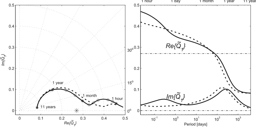
Fig. 1. Q-response of various models of mantle conductivity. The solid and dashed curves present values from realistic conductivity models representative of continental and oceanic regions, respectively. Left: polar plot of the real vs. imaginary part ofQ1. Right: Dependency of real and imaginary part ofQ1(ω)on periodT =2π/ω. The frequency-independent valueQ1=0.27 is indicated by a star (left), resp. a dashed-dotted line (right).
in Dst is one of the obstructions to improved field mod-els, and the existence of correlated low-latitude residuals in Ørsted and CHAMP residuals when using the above de-scribed approach has been clearly demonstrated (Holmeet al., 2003). The coefficientq0
1 in Eq. (1) is a measure of the strength of the axisymmetric part of the magnetospheric field forDst=0 nT, so that baseline-instabilities inDstwill result in a time-varying coefficientq10. In the present pa-per we allow for long-pa-period baseline-instabilities inDstby estimating a value ofq10for each month.
There are three main current systems contributing to the magnetospheric field (Kivelson and Russell, 1995): mag-netopause currents flowing on the magnetospheric bound-ary (magnetopause), tail currents in the neutral sheet of the geomagnetic tail, and the ring current flowing in the equa-torial plane around the Earth. Of these, the ring-current is closest to Earth (distance 3–5a). Its geometry is therefore determined more by that of Earth’s main field compared to magnetopause and -tail currents (located at distances>8a) which are more influenced by the geometry of the solar wind and the Sun-Earth connection line. Hence it is advan-tageous to use different coordinate systems for describing the various magnetospheric contributions.
Dipole/MLT coordinates are identical to solar magnetic (SM) coordinates; they are suitable for describing the mag-netic effect of the ring-current (cf. Eq. (1)), in agreement with the approach taken for the Tsyganenko models of the magnetosphere (e.g. Tsyganenko, 1990, 2002a, b). How-ever, contributions from magnetopause and tail currents are better described in the solar magnetospheric (GSM) coordi-nate system (Kivelson and Russell, 1995), which is tilted by the tilt angleψwith respect to the dipole axis (i.e., the SM z-axis). Using GSM coordinates for describing (a part of) magnetospheric contributions in geomagnetic field model-ing was introduced by Mauset al.(2005a).
Note, however, that the magnetic field observations con-tain contributions from several external current systems; it is therefore not possible to discriminate the various mag-netospheric contributions by analysis of the magnetic field at a specific time. In the following we start by modelling magnetospheric contributions in general using only the SM system; the additional use of the GSM system will be de-scribed in Section 4.
2.
Large-Scale Magnetospheric Variations and
Their Induced Counterpart
Four assumptions have to be made in deriving the last part of Eq. (1). The first assumption is that the spatial structure of the magnetospheric field can be described by spherical harmonics of degree n = 1 and order m = 0 (again, inclusion of terms with m > 0 is straightforward but will not be considered here). Hence the scalar potential describing the external field is given by
Ve(t)=a10(t)
r
a
P10(cosθd) (2)
where0
1 is the expansion coefficient of the external field and the superscript “e” stands for “external”.
The second assumption is that the time change of the magnetospheric field is proportional to that of the D st-index:10(t)= ˆq10Dst(t).
Time change of this primary (magnetospheric) field in-duces secondary currents in the conducting Earth’s interior. In the general case of a conductivity that varies in radial and horizontal direction (3-D conductivity), these induced currents produce magnetic field variations that may contain all spherical harmonic degrees and orders. In other words: although the primary, magnetospheric, field is ofP0
1 geom-etry, the secondary, induced, field contains contributionsιm n
that conductivity depends only on depth (1-D conductivity), each external coefficient induces only one internal coeffi-cient of same degreenand orderm. In that case the scalar potential describing external and induced fields (indicated by the superscript “e+i”) is
Ve+i(t)=a
In the frequency domain (time dependencyeiωt, whereωis angular frequency), this equation becomes
Ve+i(ω)=a
The assumption of a 1-D conductivity leads to a coupling of the induced (ι01) and inducing (10) coefficients. In the frequency domain the dependency is linear:
ι0
1(ω)=Q1(ω)10(ω) (5)
where Q˜1(ω)is the so calledQ-response (see Schmucker, 1985a, b, 1987 for a discussion of its properties). Multipli-cation in the frequency domain corresponds to a convolu-tion in the time domain:
ι0
where the asterisk “ ” indicates convolution. Combining Eqs. (4) and (5) yields which corresponds in the time domain to
Ve+i(t)=a
The last assumption made when deriving the third part of Eq. (1) is that mantle conductivity belongs to a very special case of 1-D models, consisting of an insulating upper man-tle and a superconductor below depthd (i.e., below radius r=c=a−d). In that case theQ-response is independent of frequencyωand is given by
Q1=
which leads to Q1 = 0.27 for a superconductor below d =1200 km depth. Since a frequency-independent value of Q1 corresponds to a delta function in the time domain, the convolution in Eq. (8) results in a multiplication:
Ve+i(t)=a10(t)·
where Q1 has been replaced by Q1 for simplicity. This equation is identical to the last part of Eq. (1). The value Q1=0.27 was found by Langel and Estes (1985a) from an analysis of Magsat data and has been widely used for de-riving field models from Ørsted and CHAMP (e.g., Olsen, 2002; Olsenet al.2000; Holmeet al., 2003).
However, Q-responses calculated from realistic models of mantle conductivity are rather different. The solid lines of Fig. 1 shows the values obtained from the mantle con-ductivity model of Schmucker (1985b), which is represen-tative for continental areas. The dashed lines are the re-sponse of “model B” of Utadaet al.(2003); this model is representative for oceanic regions. The frequency indepen-dent value of Q1 = 0.27 is shown by a dash-dotted line. The comparatively small difference between the solid and the dashed curves may be regarded as an indication of the error introduced by assuming 1-D mantle conductivity, but it is obvious that a constant value ofQ1 =0.27 (star, resp. dash-dotted line) is a rather crude approximation.
The zero imaginary part (and hence zero phase) ofQ1= 0.27 indicates that there is no time-lag between external and induced fields for the superconductor/insulator conductivity model. In contrast, the greater than zero phase of the real-istic Q-responses indicates that the induced field lags the external field. However, since the imaginary part ofQ˜1(ω) is generally much smaller than its real part, the time lag is small.
More important than the non-zero phase is the change of amplitude,| ˜Q1|, with frequency. For the realistic responses,
| ˜Q1|is larger than 0.27 for excitation periods shorter than a few months or so, but much smaller for longer periods. The induced part of long-period magnetospheric signals is therefore much more attenuated, compared to shorter peri-ods; the mantle acts as a high-pass filter. (This is contrary to the attenuation of the core field secular variation while penetratingthroughthe real conducting mantle, for which the mantle acts as a low-pass filter.) As a consequence, ex-ternal and induced fields have a different temporal behavior and should not be parameterized by the same indexDst(t). An alternative approach is described below.
3.
Decomposition of the
D
st-Index into External
and Induced Part
Dstis the north-component of the axially symmetric part of the equatorial disturbance field at the Earth’s surface caused by the magnetospheric ring-current and its induced counterpart. HenceDstcontains both external and induced contributions,
Dst(t)=Est(t)+Ist(t) (11)
The magnetic north-component at the equator at r = a is found from Eq. (3) to be Dst = X = −∂V/(a∂θ) =
−(0
1+ι01), and comparison with Eq. (11) yieldsEst= −10 andIst= −ι01.
calcu-0 5 10 15 20 25 30 35 40 45 50 55 60
0 nT 50 nT
days after June 1, 2000
D st
E
st
I
st Î
st
1960 1970 1980 1990 2000
30 25 20 15 10 5 0
[nT]
year
Î st
D st
I
st
100 101 102 103 104
101 102 103 104 105 106
1 y
ear
6 months
1 month
27 da
ys
13.5 da
ys
9 da
ys
1 da
y
period in days
nT
2/cpd
D st
Est
Î st
I
st
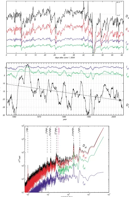
Fig. 2. Top: Time series ofDst(black)Est(red) andIst(blue), for June and July 2000. The green curve showsIˆst=Dst·Q1(/1+Q1)=0.21Dst(t); the value traditionally used for describing the time-changes of induced contributions. Bottom: One-year moving averages for the years 1957–2004. The dashed lines present linear trend estimates. Bottom: Power spectrum (in units of nT2/cpd, where cpd stands for “cycles per day”) ofD
lated for all considered frequencies using a given model of transformed back to the time domain to obtain Ist(t), and Est(t)=Dst(t)−Ist(t)is calculated.
As an example, the top panel of Fig. 2 shows two months of Dst (black curve) and its constituents Est (red) and Ist (blue), separated using the conductivity model of Utadaet al.(2003). (It is expected that use of a different, but realis-tic, conductivity model only results in small changes.) The dotted lines indicate the respective zero-levels. Separation ofDstusing a constant (frequency independent) value ofQ1 yieldsDst(t)= ˆEst(t)+ ˆIst(t)with
Proper handling of long-term variations in the induced fields (whether real or spurious) is essential for deriving good field models; errors will influence estimates of the main-field coefficientg0
1and its time change. The presence of long-term fluctuations in Dstcan be studied by looking at 1-year moving averages, presented in the middle part of Fig. 2. The black curve shows the 1-year average of Dst; the blue and green curve present in the same way processedIstandIˆst. Applying a one-year moving average smooths much of the time-changes of Dst; however, the smoothed time-series reveals a large number of spikes, steps and excursions, which occur preferentially at the turn of the years. This is due to the way the index is calculated (definition of the baseline by polynomials over a few years) and indicates that the baseline ofDstmight not be constant in time.
Note the non-zero offset of Dst. This offset, though reduced in size, is also present in Iˆst, due to the assumed proportionality with Dst. However, a static induced field (offset) is unphysical, and hence its presence indicates an error that will be introduced by assuming a constant value of Q1. Using proper (frequency dependent) values of the Q-response, the offset disappears, as indicated by the zero mean ofIst.
The bottom panel of Fig. 2 shows the power spectra of the various indices. The well known periodicities of geo-magnetic activity (annual and semi-annual periods, 27-day solar rotation period and its harmonics, daily period) are clearly seen. Surprisingly, there is also a peak at a period of 1 month (indicated by the magenta vertical line), which may be an artifact introduced during the calculation ofDst. The induced part,Ist, obtained using a realistic Earth model has more than 10 times (100 times) less power for periods longer than 1 year (8 years) compared to the signal obtained
with a fixedQ-value (i.e., Iˆst), becauseIstis much less in-fluenced by baseline instabilities inDstthan is Iˆst.
SinceIˆstis traditionally used to parameterize internal (in-duced) contributions, the data are forced to fit an unphysical internal dipole field of a few nT size. This results in main field coefficientsg0
1 that are biased (too low) by a value of equal size but opposite sign.
Moreover, there is an obvious trend of about−0.15 nT/yr in Dst, and a somewhat smaller trend in Iˆst (see middle panel of Fig. 2). However, the trend is much larger during the last years, and when data covering only the last five years are analyzed (Ørsted and CHAMP period), the trend is about−1 nT/yr in Dstand about−0.2 nT/yr in Iˆst. Use ofIˆstto parameterize internal fields will therefore result in a secular variation (SV) coefficientg˙0
1that is biased (too low) by about 0.2 nT/yr; this is confirmed by field modeling, as demonstrated in the next section.
Separation ofDstinto external and induced parts allows us to parameterize external and induced field contributions in a more appropriate way compared to the usual approach shown in the last term of Eq. (1) and Eq. (10). We instead parameterize external fields byEst(t)and induced fields by Ist(t), and use instead of the last line of Eq. (1), where both the external and induced fields are taken proportional toDst(t).
4.
Application: Estimation of New Field Models
The above-described new parameterization of external and induced fields has been applied to more than 5 years of satellite data from the Ørsted and CHAMP satellites. Data selection and model parameterization follows closely that of previous models like the OSVM (Olsen, 2002).We use Ørsted scalar and vector data between March 1999 and September 2004, and CHAMP scalar data be-tween August 2000 and August 2004. We use the K p in-dex to restrict the data to quiet times, specifically requiring K p ≤ 1+ for the time of observation and K p ≤ 2o for the previous three hour interval. Contrary to previous mod-els, we do not select data according to the absolute value of the Dst index (since the baseline of Dstis not constant; for instance during the first half of 2003 Dst is probably off by 15 nT, as discussed later). However, we require that Dstdoes not change by more than 1 nT/hr. Only data from dark regions (sun 5◦ below horizon) were used, to reduce contributions from ionospheric currents at middle and low latitudes. The effect of polar cap ionospheric currents is minimized by excluding data in the polar caps for which the dawn-dusk component of the interplanetary magnetic field was|By|>3 nT. Ørsted vector data have been taken
for dipole latitudes equatorward of±60o, scalar data were used for regions poleward of±60o or if attitude data were not available. Sampling interval was 60 seconds; weights
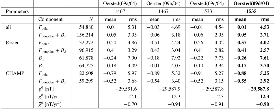
inver-Table 1. NumberNof data points as well as mean and rms (in nT) for the four derived models: Oersted(09a/04): derived using the “classical” approach of describing induced contributions (Eq. (10))
Oersted(09b/04): as Oersted(09a/04), but derived using the new approach of describing induced contributions (Eq. (14)) Oersted(09c/04): as Oersted(09b/04), but solving for a time-varyingq0
1(t)
Oersted(09d/04): as Oersted(09c/04), but including the two external coefficientsq10,GSMandq20,GSMin GSM coordinates
Oersted(09a/04) Oersted(09b/04) Oersted(09c/04) Oersted(09d/04)
Parameters 1467 1467 1533 1535
Component N mean rms mean rms mean rms mean rms
all Fpolar 54,880 0.01 5.31 −0.03 4.69 −0.01 4.54 0.01 4.53
Fnonpolar+BB 156,214 0.05 3.95 0.06 3.18 0.06 2.95 0.05 2.71
Ørsted Fpolar 32,272 0.50 4.86 0.51 4.24 0.56 4.02 0.57 4.02
Fnonpolar+BB 96,915 0.41 3.29 0.43 3.04 0.41 2.82 0.41 2.57
B⊥ 61,878 −0.24 7.90 −0.18 7.92 −0.22 7.73 −0.26 7.61 B3 64,725 −0.18 4.09 −0.01 4.07 −0.10 3.94 −0.17 3.70 CHAMP Fpolar 22,608 −0.79 5.97 −0.89 5.32 −0.91 5.27 −0.88 5.25 Fnonpolar+BB 59,299 −0.52 3.68 −0.54 3.40 −0.52 3.15 −0.55 2.92 g0
1[nT] −29,591.6 −29,587.9 −29,587.8 −29,587.8
˙
g0
1[nT/yr] 12.1 12.3 12.3 12.3
¨
g0 1[nT/yr
2] −0.70 −0.94 −0.91 −0.90
sion (Holme and Bloxham, 1996; Holme, 2000). Since we are mostly interested in spherical harmonic coefficients de-scribing core and long-wavelength lithospheric fields, we have subtracted the short-wavelength (n>30) lithospheric field as given by CM4 (Sabakaet al., 2004) from all obser-vations.
Following Eq. (1), the time dependence of the internal Gauss coefficients{gm
n(t),hmn(t)}are expanded in a Taylor
series according to
gm
n(t)=gnm+(t−t0)· ˙gnm+ 1 2(t−t0)
2· ¨gm
n forn=1−8
=gm
n +(t−t0)· ˙gnm forn=9−16
=gm
n (const.) forn=17−32 (15) and similar for the coefficientshmn(t).t0=2002.0 is model epoch. This yields 1088 static coefficients (up to degree and orderNstatic=32), 288 coefficients of secular variation (up to NSV = 16), and 80 coefficients of secular acceleration (up toNSA=8).
As for the OSVM, external coefficients{qm
n,snm}are
es-timated up to degree Next = 2 (which gives 8 coeffi-cients). However, contrary to previous models we use dipole-colatitude/MLT coordinates, θd,Tm (instead of
co-latitude and longitude).
Several models were derived, using the same data and (almost the same) number of model parameters. The only difference between the first two models is that the classi-cal approach of treating magnetospheric and induced fields using Dst and a fixed value Q1 = 0.27 (Eq. (10), but for m = 0,1) was used for deriving the first model, called Oersted(09a/04) while for the second model, called Oer-sted(09b/04), the new approach (Eq. (14), but form=0,1) was used, i.e. external fields are parameterized byEstwhile their internal, induced counterparts are parameterized byIst. In both cases, 3 coefficients of proportionality (qˆ0
1,qˆ11,sˆ10, or
ˇ
q0
1,qˇ11,sˇ01) are estimated.
In total, each model has 1467 free parameters (1456 in-ternal coefficients describing the static field, secular varia-tion and secular acceleravaria-tion, 8 static external coefficients, 3 coefficients ofDst/Est/Ist-dependency).
Table 1 shows the statistics of the models. The new parameterization (Eq. (14)) reduces the model misfit by up to 25% (for the scalar misfit at non-polar latitudes), compared to using the “classical” approach (Eq. (10)). Note that the number of parameters is the same for both models. Also listed are the values of the main coefficient g01 and of its first and second time derivative. g01 of the second model, Oersted(09b/04), is 3.7 nT less negative than the corresponding value of model Oersted(09a/04), and g˙0
1 is larger by 0.2 nT/yr, in agreement with the predictions made in the previous section.
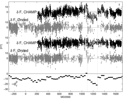
Fig. 3. Low-latitude (<±10odip-latitude) scalar residuals as a function of time (day after midnight, 1/1/2000) with respect to model Oersted(09a/04) (upper part) and Oersted(09d/04) (middle part). Also shown is−q0
1(t)of model Oersted(09d/04) (lower part). Horizontal lines represent zero-levels.
used after March 1, 2004. The observed large offset after day count 1100 is probably because the finalDstindex was not available for 2003 onward.
To investigate this, we derived a third model, called Oer-sted(09c/04) where we allow the “static” external coeffi-cient q10 (cf. the second term of Eq. (1)) to change with time. We do this by estimating 67 values ofq0
1, one for each month of the data window (March 1999–September 2004). The lower part of Fig. 3 shows these values of−q0
1, together with time series of the low-latitude scalar residuals with re-spect to that model. (At the equator, the magnetic intensity of a P0
1 source field is proportional to−q10, which is the reason for choosing the negative sign.) There is a consider-able variation; the time-change ofq0
1 suggests for instance that Dst is off by about 15 nT during the first 6 months of 2003 (indicated by the dashed vertical lines). The misfit of that model is slightly smaller (reduction of non-polar scalar misfit of 7%) compared to the second model; however, one has to keep in mind that the number of model parameters has increased by 66 (4%). Co-estimation of a Dstoffset on a monthly basis, as done here, removes most of the corre-lated low-latitude residuals, as can be seen when comparing the two upper and the middle part of Fig. 3.
Contrary to previous models like OSVM, the present models do not incorporate annual and semi-annual vari-ations (solving for an annual and semi-annual variation of q0
1 would be in conflict with the explicit determination
of monthly values forq10, described in the previous para-graph). However, as mentioned before, currents in the mag-netopause and tail are better described in the GSM coor-dinate system; a field which is constant in GSM coordi-nates has seasonal and daily variations in an Earth-fixed coordinate system. To investigate the effect of including GSM-coefficients we derived a fourth model, called Oer-sted(09d/04). It is identical to model Oersted(09c/04) but includes also the two coefficients q10,GSM andq20,GSM de-scribing daily and seasonal field variations, as seen in the dipole coordinate system, of a magnetospheric field which is constant in the GSM system. The total number of pa-rameters of that model is thus 1535 (1456 static internal coefficients; 7 static external coefficients in the SM coordi-nate system; 67 external SM coefficientsq10 (one for each month); 3 coefficients of Ist/Est dependency; 2 external GSM-coefficients). Table 1 shows that the model misfit of that last model is further decreased (scalar misfit at non-polar latitudes is about 9% lower compared to model Oer-sted(09c/04)), although that last model only solves for two additional parameters.
5.
Discussion
10 15 20 25 30 101
102
degree n
[nT
2]
a d CM4 MF4
10 15 20 25 30
0.75 0.8 0.85 0.9 0.95 1
degree n
deg
ree correlation
ρn
d / CM4 d / MF4 CM4 / MF4
0 2 4 6 8 10 12 14 16 101
100 101 102 103
degree n
[(nT/yr)
2] or [(nT/yr
2)
2]
secular variation (linear)
secular acceleration (quadratic)
a d CM4
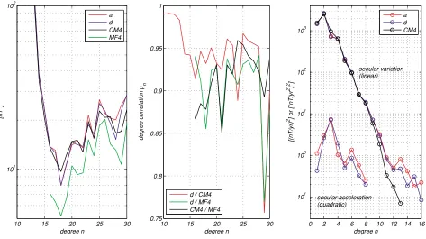
Fig. 4. Left: Power spectra of the static field part of various models. Middle: Degree correlation between the static part of the models. Right: Power spectra of secular variation and secular acceleration, respectively.
09d in comparison with that of CM4 (Sabakaet al., 2004) and MF4 (Mauset al., 2005b). Note that MF4 is a model of the crustal field only, and therfore contains only coefficients with degreen ≥16. The three models 09a, 09d and CM4 have roughly the same power, while MF4 has considerably less power, partly due to the use of a track-by-track filtering of the data when deriving MF4.
The middle panel shows degree correlation,ρn, between
the static part of the models 09d, CM4 and MF4. There is consistently higher correlation between models 09d and CM4 compared to MF4. The right panel shows the power spectra of the linear and quadratic time changes (secular variation and acceleration, respectively). With the excep-tion of secular acceleraexcep-tion at degree n = 1, model 09d contains less power compared to model 09a, which may in-dicate that the coefficients of model 09a are more strongly influenced by unmodeled signals than those of model 09d. Also shown is secular variation of CM4 for epoch 2002.0. Note that CM4 is regularized, which is the reason for the faster decrease of power above degree 8 or so.
The complexity of modeling magnetospheric contribu-tions increases from model Oersted(09a/04) to model 09d, and it is interesting to investigate how this affectsq0
1, the main coefficient of magnetospheric contributions. The static coefficientq10 changes from 20.2 nT to 16.7 nT be-tween model 09a and 09b; this change is probably mainly due to use of Est instead of Dst (which should decrease the coefficient by a factor of 0.79). The mean value of the (now time-dependent) coefficient q10 of model 09c is q10 =17.2 nT, in good agreement with the value of model 09b. As for model 09d, the sum of the magnetospheric contributions in SM and GSM coordinates is very similar
to that value: q10 +g01,GSM = 17.4 nT; however, about one half is constant wrt the dipole (SM) coordinate system (q10 =9.1 nT), while the other half is constant in the GSM coordinate system (g01,GSM = 8.3 nT). All other external coefficients have amplitudes well below 1 nT, with the ex-ception ofq21, which is between−1.1 nT (model 09b) and
−1.5 nT (model 09d).
As pointed out by Mauset al.(2005a) and Maus and L¨uhr (2005), modeling magnetospheric fields in the GSM coordi-nate system introduces some seasonal and daily variations in an Earth-fixed system, due to the time changes of the dipole-tiltψ. Secondary currents are therefore induced in the Earth’s interior which, however, are not considered in the presented models; they are expected to have amplitudes below 1 nT.
6.
Extraction of the IGRF 2005 Candidate Models
Our candidate model IGRF-A1 is an N = 13 trunca-tion of model Oersted(09d/04), propagated to epoch 2005.0 (using linear as well as quadratic terms). The same correc-tion for ionospheric leakage that we used for our candidate model for DGRF2000 (cf., Olsenet al., 2005), based on the work of Lowes and Olsen (2004), has been applied, and the formal standard deviations of the coefficients have been scaled by the same empirical factors.Two candidate models for secular variation have been derived from model Oersted(09d/04): SV-A1-2005 is the N =8 truncation of the secular variation after propagation to epoch 2005.0, while SV-A3-2007.5 is the N = 8 trun-cation of the secular variation after propagation to epoch 2007.5. Both propagations were performed using linear as well as quadratic terms.
panel of Fig. 4 peaks at degree n = 3; this peak is due to a rather large value for the coefficienth¨3
3 = 1.2 nT/yr2. For the extraction of the IGRF candidates we have to ex-trapolate the coefficients from model epocht0 =2002.0 to epoch 2005.0 (for the main field) and 2007.5 (for the secu-lar variation), respectively. Since a quadratic extrapolation is problematic, we decided to derive an additional model, Oersted(09g/04), without quadratic terms. Only data from one year (August 2003–September 2004) were used; data selection and model parameterization is similar to that used for model Oersted(09a/04), but the model epoch is 2005.0, truncation level of the secular variation isNSV =13, and no
quadratic time terms were derived (NS A =0). TheN =13
truncation of that model, after correcting for ionospheric leakage, is our second main field candidate, called IGRF-A2. Likewise, another secular variation candidate, SV-A2-2005, is derived as theN =8 truncation of the secular vari-ation of model Oersted(09g/04). However, we derived these two candidate models (IGRF-A2 and SV-A2-2005) mainly for evaluation purposes; candidate model IGRF-A1 is our preferred candidate for the main field, and SV-A3-2007.5 is our preferred candidate for secular variation.
References
Holme, R., Modelling of attitude error in vector magnetic data: application to Ørsted data,Earth Planets Space,52, 1187–1197, 2000.
Holme, R. and J. Bloxham, The treatment of attitude errors in satellite geomagnetic data,Phys. Earth Planet. Int.,98, 221–233, 1996. Holme, R., N. Olsen, M. Rother, and H. L¨uhr, CO2: A CHAMP magnetic
field model, inFirst CHAMP Mission results for Gravity, Magnetic and Atmospheric Studies, edited by C. Reigber, H. L¨uhr, and P. Schwintzer, pp. 220–225, Springer Verlag, 2003.
Kivelson, M. G. and C. T. Russell,Introduction to Space Physics, Cam-bridge University Press, 1995.
Langel, R. A. and R. H. Estes, Large-scale, near-Earth magnetic fields from external sources and the corresponding induced internal field,J. Geophys. Res.,90, 2487–2494, 1985a.
Langel, R. A. and R. H. Estes, The near-Earth magnetic field at 1980 de-termined from MAGSAT data,J. Geophys. Res.,90, 2495–2509, 1985b. Langel, R. A. and W. J. Hinze,The Magnetic Field of the Earth’s Litho-sphere: The Satellite Perspective, Cambridge University Press, 1998. Langel, R. A., G. D. Mead, E. R. Lancaster, R. H. Estes, and E. B. Fabiano,
Initial geomagnetic field model from Magsat vector data,Geophys. Res. Lett.,7, 793–796, 1980.
Lowes, F. J. and N. Olsen, A more realistic estimate of the variances and systematic errors in spherical harmonic geomagnetic field models,
Geophys. J. Int.,157, 1027–1044, 2004.
Maus, S. and H. L¨uhr, Signature of the quiet-time magnetospheric mag-netic field and its electromagmag-netic induction in the rotating Earth, Geo-phys. J. Int.,162, 755–763, 2005.
Maus, S. and P. Weidelt, Separating the magnetospheric disturbance mag-netic field into external and transient internal contributions using a 1D conductivity model of the Earth, Geophys. Res. Lett.,31, L12,614, doi:10.1029/2004GL020,232, 2004.
Maus, S., H. L¨uhr, G. Balasis, M. Rother, and M. Mandea, Introducing POMME, the POtsdam Magnetic Model of the Earth, inEarth Observa-tion with CHAMP, Results from Three Years in Orbit, edited by C. Reig-ber, H. L¨uhr, P. Schwintzer, and J. Wickert, pp. 293–298, Springer Ver-lag, 2005a.
Maus, S., M. Rother, K. Hemant, H. L¨uhr, A. V. Kuvshinov, and N. Olsen, Earth’s crustal magnetic field determined to spherical harmonic degree 90 from CHAMP satellite measurements,Geophys. J. Int., 2005b (sub-mitted).
Olsen, N., A model of the geomagnetic field and its secular variation for epoch 2000 estimated from Ørsted data,Geophys. J. Int.,149, 454–462, 2002.
Olsen, N., New parameterization of external and induced fields in geomag-netic field modeling,Geophysical Research Abstracts,6, 02,454, 2004. Olsen, N., T. J. Sabaka, and L. Tøffner-Clausen, Determination of the
IGRF 2000 model,Earth Planets Space,52, 1175–1182, 2000. Olsen, N., F. Lowes, and T. J. Sabaka, Ionospheric and induced field
leak-age in geomagnetic field models, and derivation of candidate models for DGRF 1995 and DGRF 2000,Earth Planets Space,57, this issue, 1191–1196, 2005.
Sabaka, T. J., N. Olsen, and M. Purucker, Extending comprehensive mod-els of the Earth’s magnetic field with Ørsted and CHAMP data, Geo-phys. J. Int.,159, 521–547, doi: 10.1111/j.1365–246X.2004.02,421.x, 2004.
Schmucker, U., Magnetic and electric fields due to electromagnetic induc-tion by external sources, inLandolt-B¨ornstein, New-Series, 5/2b, pp. 100–125, Springer-Verlag, Berlin-Heidelberg, 1985a.
Schmucker, U., Electrical properties of the Earth’s interior, in Landolt-B¨ornstein, New-Series, 5/2b, pp. 370–397, Springer-Verlag, Berlin-Heidelberg, 1985b.
Schmucker, U., Substitute conductors for electromagnetic response esti-mates,PAGEOPH,125, 341–367, 1987.
Tsyganenko, N. A., Quantitative models of the magnetospheric magnetic field: methods and results,Space Sci. Rev.,54, 75–186, 1990. Tsyganenko, N. A., A model of the near magnetosphere with a
dawn-dusk asymmetry 1. Mathematical structure,J. Geophys. Res.,107, 12–1, 2002a.
Tsyganenko, N. A., A model of the near magnetosphere with a dawn-dusk asymmetry 2. Parameterization and fitting to observations,J. Geophys. Res.,107, 10–1, 2002b.
Utada, H., T. Koyama, H. Shimizu, and A. D. Chave, A semi-global reference model for electrical conductivity in the mid-mantle be-neath the north Pacific region, Geophys. Res. Lett., 30, 43–1, DOI 10.1029/2002GL016,092, 2003.