A Deregulated Optimal Power System Using
Flexible Real Coded Biogeography-Based
Optimization
P. Vinothini Sahayam1, A. Josephine Amala2
PG Student [PSE], Dept. of EEE, JJ College of Engineering, Tiruchirappalli, Tamilnadu, India1 Professor, Dept. of EEE, JJ College of Engineering, Tiruchirappalli, Tamilnadu, India2
ABSTRACT: This paper presents a biogeography-based optimization based algorithm for solving constrained optimal power flow problems in power systems. In this paper, we extend the original BBO and present a flexible real-coded BBO approach, referred to as FRCBBO, for the global optimization problems in the deregulated power system. Using flexible real coded biogeography-based optimization (FRCBBO), we present the optimization of various objective functions of an optimal power flow (OPF) problem in a power system. We aimed to determine the optimal settings of control variables for an OPF problem. The proposed approach was tested on a standard IEEE 30-bus system and an IEEE 57-bus system with different objective functions. The results indicate the good performance of the proposed FRCBBO method.
KEYWORDS: Optimal power flow, Biogeography-based optimization, Fuel cost, Voltage profile, Voltage stability.
I.INTRODUCTION
Biogeography-based optimization (BBO) is a new optimization algorithm, and, thus far, it has been used in power system optimization. The application of biogeography to optimization was first presented in 10], and it describes how a natural process can be modelled to solve general optimization problems. BBO maintains its set of solution from one iteration to the next, although the characteristics change as the algorithm progresses. BBO has many features in common with the PSO algorithm. In PSO, solutions are maintained from one iteration to the next, but each solution is able to learn from its neighbours and adapt itself as the algorithm progresses. However, PSO solutions do not change directly; first, their velocities are changed, then positions change.
II. RELATED WORKS
The power of flexible real coded biogeography-based optimization (FRCBBO) to solve the OPF problem is discussed in this paper.
T
he BBO algorithm has been employed to IEEE 30-bus, IEEE 57-bus systems having linear operating constraint. The same three objective functions are used in this study, namely, minimization of fuel cost, improvement of voltage profile, and improvement of voltage stability. In the FRCBBO approach, therefore, an adaptive Gaussian mutation is integrated into the OPF problem, thereby avoiding premature convergence, improving population diversity, and enhancing the exploration ability.III. PROBLEM FORMULATION
Generally, an OPF problem is a large-scale, highly constrained nonlinear optimization problem. It may be defined as:
minf(x, u) (1)
subjecttog(x, u) = 0 (2)
h((x, u)≤0 (3)
Where f is the objective function to be minimized, x and u are the vectors of dependent and independent control variables, respectively, g is the equality constraint, and h is the operating inequality constraint. The vector of dependent variables can be represented as:
X = P , V … V , Q … Q , S … S (4)
Where PG1 denotes the slack bus power; VL denotes the load bus voltage; QG denotes the reactive power output of the
generator; SL denotes the transmission line flow; Npq is the number of load buses; Ng is the number of
voltage-controlled buses and Nl is the number of transmission lines. The vector of independent control variables can be represented as:
u = P … P , V … V , T … T , Q … Q (5)
Where PG is the active power output of generators; VG is the voltage at the voltage-controlled bus; T is the tap setting of
the tap-changing transformer; and QC is the output of shunt VAR compensators; Nt and Nc are the number of
tap-changing transformers and shunt VAR compensators, respectively.
Equality constraints (g)
P −P − ∑ V V [G cos(δ − δ) + B sin(δ − δ)] = 0 i = 1,2, … … Nb (6)
Q −Q − ∑ V V [G sin(δ − δ) + B cos(δ − δ)] = 0 i = 1,2, … … Nb (7)
Where PGi and QGi are the injected active and reactive power at ith bus, respectively; PDi and QDi are the demanded
active and reactive power at ith bus, respectively; Vi and Vj are the magnitude of voltage at ith and jth bus, respectively;
Gij and Bij are the real and imaginary part of the admittance of line connected between ith and jth bus; δ and δ are the
phase angle of voltage at ith and jth bus, respectively; Nb is the number of buses.
Inequality constraints (h)
(i)Generator constraints: The generator active and reactive power outputs and voltage are restricted by their upper and lower limits.
P ≤P ≤P i = 1,2, … … Ng (8)
Q ≤Q ≤Q i = 1,2, … … Ng (9)
V ≤V ≤Q i = 1,2, … … Ng (10)
(ii) Transformer constraints: Tap-changing transformers have minimum and maximum setting limits:
(iii) Switchable VAR sources: These have minimum and maximum limits:
Q ≤Q ≤Q i = 1,2, . . Nc (12)
(iv) Security constraints: These include the limits on load bus voltage and transmission line flow.
V ≤V ≤V i = 1,2, … Npq (13)
MVA ≤MVA (14)
Where MVAk is the power flow at kth line; MVAkmax is the power flow capacity of kth transmission line. Finally, the
objective function with all constraints combined for the OPF problem.
IV. BIOGEOGRAPHY-BASED OPTIMIZATION
Dan [11] proposed a comprehensive algorithm (BBO) for solving optimization problems based on the study of geographical distribution of species. A BBO algorithm has two main operators: migration operator and mutation operator.
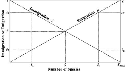
Fig. 1 Model of immigration and emigration probabilities.
A. Migration operator
Migration is a process of probabilistically modifying each individual in the habitat randomly. A geographical area with high habitat suitability index (HSI) tends to have a large number of species, high emigration rate, and low immigration rate. Suitability index variables (SIVs) define the characteristics of a habitat. A habitat with a high HSI tends to be more static in its species distribution. Such an habitat signifies a good solution in terms of an optimization problem. Immigration rate, ⋋ , and emigration rate, μ , are functions of the number of species in a habitat. For a habitat with no species, its immigration rate can be the highest. ⋋ is given by
⋋ =I 1− (15)
Where I is the maximum possible immigration rate, k is the number of species of kth individual, and n is the maximum number of species. , μ is given by:
μ = E (16)
Where E is the maximum possible emigration rate. B. Mutation operator
Mutation tends to increase the diversity of a species in a habitat. Due to natural events, the HSI of a habitat can change dramatically, causing the species count to shift away from its equilibrium value. Species count may be a probability value (Pi). If this probability value is very low, an individual solution is thought to have beenmutated with other
solutions. So, the mutation rate of an individual solution can be calculated using species count probability, given by:
Where Mi is the mutation rate, Mmax is the maximum mutation rate, which is a user-defined parameter, and Pmax is the
maximum probability of species count. In BBO, a mutation characteristic function is given by:
X′ = X + rand (0.1) × X −X (18)
Where Xi is the decision variable; Ximax andXimin are the lower and upper limits of the decision variable, respectively.
V. FLEXIBLE REAL CODED BIOGEOGRAPHY-BASED OPTIMIZATION
RCBBO was proposed by Gong et al. [12] as an extension to BBO. In RCBBO, individuals are represented by a D-dimensional real parameter vector, and a probabilistically based Gaussian mutation is used. The Gaussian mutation characteristic function is given by:
X′ = X + N (µσ ) (19)
WhereN = (μ,σ )represents the Gaussian random variable with mean l and varianceσ . The values of mean and variance are considered 0 and 1, respectively.Generally, a probability-based mutation operation is known to improve the convergence characteristics. Therefore, adaptive Gaussian mutation is applied in the present work to improve the solution of a worst half set of habitats in the population. In Eq. (19), μ= 0, and σ is found using the following equation:
σ= β×∑ × X −X (20)
Whereβ the scaling factor or mutation probability, Fi is the fitness value of ith individual, and f min is the minimum
fitness value of the habitat in the population. Adaptive mutation probability is given by:
β = β - × T (21)
Whereβ = 1, β =0:005, Tmax is the maximum iteration, and T is the current iteration. The use of adaptive mutation can prevent premature convergence, thereby producing a smooth convergence. This method of mutation can be easily used with real-coded variables, which have been widely used in EP, and hence to carry out local as well as global searches. The steps for solving the OPF problem using proposed FRCBBO is as follows:
Step 1: Initialization
Habitat modification probability (Pmod), minimum and maximum values of adaptive mutation probability
(β andβ ), maximum immigration and emigration rates for each island, maximum species count (P), and maximum iterations are initialized.
Step 2: Generate SIVs for the habitat randomly within the feasible region. Individuals (control variables) in the habitats are initialized as:
X = X + rand(0.1) × X −X (22)
where i =1, 2, ... , P and j =1, 2, ... , Nvar; Nvar is the number of control variables; Xjmax and Xjmin are the
upper and lower limits of jth control variable.
Step 3: Perform load flow analysis using Newton–Raphson method and determine the dependent variables (Eq. 4). Compute the fitness value (HSI) for each habitat set.
Step 4: Based on the HSI value, elite habitats are identified. Step 5: Iterative algorithm for optimization:
Perform migration operation on SIVs of each non-elite habitat selected for migration.
Calculate immigration and emigration rates for each habitat set, using Eqs. (15) and (16).
Update the habitat set after migration operation.
Recalculate the HSI value of modified habitat set; feasibility of the solution is verified and habitat set sorted based on new HSI value.
σ =× × P −P , i=2,3, . . . Ng (23)
Where Fij is the fuel cost of ith generator (individual) of jth habitat; f min is the minimum fitness value of the habitat in
the population; P Gimax and P Gi min are the maximum and minimum limits of active power generation of ith generator.
Fuel cost minimization is the main objective function for all case studies, fuel cost mainly depends on active power generation; each active power control variable contributes to minimize the fuel cost individually. So,σ for active power control variables is calculated individually from the fuel cost of each active power generation. But other control variables (except active power control variables) are not directly related to fuel cost minimization function; they are used to satisfy the constraints of the OPF problem. So σ for other control variables is calculated using the fitness value (Fj)of the jth habitat set (not individuals of habitat).
σ = β× × X – X
i = Ng + 1. Ng + 2 … . . Nvar (24)
Where Fj is the fitness value of jth habitat; Ximax and Ximin are the maximum and minimum limits of ith individual.
Compute the fitness value (HSI) for each habitat set after mutation operation and verify the feasibility of the solution.
Sort the habitat set based on new HSI value.
Stop the iteration counter if the maximum number of iterations is reached.
Step 6: Finally SIVs should satisfy the objective function as well as constraints of the problem.
VI. RESULTS AND DISCUSSION
The power of the FRCBBO algorithm to solve the OPF problem was tested using an IEEE 30-bus and an IEEE 57-bus systems. All simulations were performed on a personal computer (i3 3.1 GHz Intel Processor and 2 GB RAM running MATLAB R2013a).
A. IEEE 30-bus system
An IEEE 30-bus system has six generators, four tap-changing transformers, and nine shunt VAR compensation buses for reactive power control. The system active power demand is 283.4 MW and reactive power demand is 126.2 MVAR at 100 MVA base. The magnitude of voltage limits for generator buses are 0.95–1.1 p.u. and for load buses are 0.95–1.05 p.u. Bus 1 is taken as the slack bus.
The bus data and line data [13] and the minimum and maximum limits for control variables [14] are obtained from literature. The optimal control parameters for the algorithm are obtained by number of simulation results. They are: habitat size = 50, habitat modification probability = 1, immigration probability = 1, step size for numerical integration = 1, maximum immigration and emigration rate = 1, mutation probability = 0.005 and maximum number of iterations = 200.
Case 1: Minimization of fuel cost
It represents the quadratic cost function whose objective function is expressed as follows: f=FC=∑ (a + b × P + c P ) (25)
Where FC is the total fuel cost; ai; bi and ci are fuel cost coefficients of the ith unit. The quadratic cost coefficients are
0 20 40 60 80 100 120 140 160 180 200 0
1000 2000 3000 4000 5000 6000
Generation
M
in
im
u
m
C
o
s
t
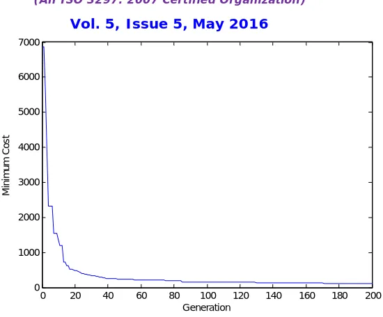
Fig. 1. Convergence characteristics of proposed FRCBBO
Results across different optimization techniques. The first three rows mentioned in the table are obtained from our own implementation of algorithms; i.e. original BBO [15] and RCBBO [16]. Best fuel cost obtained by the proposed FRCBBO was 800.5159 $/h, and average fuel cost was 800.6412 $/h. Table-1 shows the convergence characteristics of optimization methods, considered in this work are depicted in Fig. 1, which indicates premature convergence in FRCBBO
Table: 1 Minimization of Fuel Cost
Case 2: Voltage profile improvement
This objective function minimizes the fuel cost while enhancing the voltage profile by minimizing all the load bus voltage deviation from 1.0 p.u. It can be expressed as:
f = (a + b × P + C × P ) + ⋋ |V −1.0| (26)
Where⋋ is a weighting factor selected by the user, the sum of voltage deviation in this case is 0.0920, which was 0.8867 in the previous case. Hence there is an improvement from 89.62% in the voltage profile. The results of this objective function across different optimization methods considered. Table-2 shows the proposed FRCBBO shows a better solution than other. The best solution is infeasible because the reactive power of the slack bus is 20.1144, in violation of the limits reported.
Table: 2 Voltage Profile Improvements
BUS SYSTEM FUEL COST ($/h)
BEST AVERAGE WORST
IEEE 30 700.5159 700.6412 700.9262
IEEE 57 41686 41718 41737
BUS SYSTEM VOLTAGE DEVIATION(p.u)
BEST AVERAGE WORST
IEEE 30 0.095 0.1008 0.011
Case 3: Enhancement of voltage stability
Voltage stability is the ability of a power system to maintain acceptable voltages at all buses in the system under normal conditions. A system enters a state of voltage instability when a disturbance, such as an increase in load demand or change in system condition, causes a progressive and an uncontrollable decrease in voltage. Table-3 shows voltage stability is an important parameter in a power system operation. It can be defined via minimizing the voltage stability indicator (L-index) values of each bus of a power system. The L-index of a bus specifies the proximity of the voltage collapse condition of that bus. The L-index of a jth load bus is defined as:
L = 1− F V
V (27)
j = 1,2, … Npq (28)
F = −[Y ] [Y ] (29)
Where Vi is the voltage of the ith generator bus and Vj is the voltage of the jth load bus. Y1 and Y2is the sub matrices of
the system Ybus obtained after separating the load and generator buses parameter. Lj equal to one represents the
voltage collapse condition of jth bus. So, a global power system’s L-index is given as: L = max (L j) j = 1, 2, ... ,Npq (30)
A lower value of L-index represents a more stable system. An objective function combining minimization of fuel cost and enhancement of voltage stability is suggested by minimizing the L-index value. The results of this objective function across different optimization methods considered are presented. The best solutions are infeasible because the voltage magnitudes at most of the load buses are greater than 1.05 p.u., which violate their limits reported in [17].
Table: 3 Enhancement of Voltage Stability
VII.CONCLUSION
Using case studies approach, FRCBBO has been implemented successfully in different power systems for congestion management. This algorithm is ideal for independent system operators to solve different objective functions in deregulated environments. Our simulation results suggest that the proposed FRCBBO approach is able to improve exploration ability and diversity of the population, in addition to yielding good convergence characteristics and robustness, as with other heuristic algorithms. The present work adds further evidence to suggest that the proposed FRCBBO is the best to solve nonlinear objective functions, with its ability to prevent premature convergence of solutions. The objectives of fuel cost minimization, voltage profile and voltage stability enhancement under intact and contingency conditions were successfully tested using this approach. The results of the problem are compared against literature results obtained using different optimization methods.
REFERENCES
[1] Dommel, H. W., and Tinney, W. F., “Optimal power flow solutions,” IEEE Trans. Power Syst. Apparatus Syst., Vol. PAS-87, No. 10, pp. 1866–1876, 1968.
[2] Momoh, J. A., Adapa, R., and El-Hawary, M. E., “A review of selected optimal power flow literature to 1993. I. Nonlinear and quadratic programming approaches,” IEEE Trans. Power Syst., Vol. 14, No. 1, pp. 96–104, 1999.
[3] Gaing, Z., and Huang, H. S., “Real-coded mixed integer genetic algorithm for constrained optimal power flow,” IEEE TENCON Region 10 Conf., Vol. 3, pp. 323–326, November 2004.
[4] Roa-Sepulveda, C. A., and Pavez-Lazo, B. J., “A solution to the optimal power flow using simulated annealing,” IEEE Porto Power Tech. Proc., Vol. 2, pp. 1–5, 2001.
BUS SYSTEM ENHANCEMENT OF VOLTAGE STABILITY
BEST AVERAGE WORST
IEEE 30 0.141 0.1375 0.151
[5] AlRashidi, M. R., and El-Hawary, M. E., “Hybrid particle swarm optimization approach for solving the discrete OPF problem considering the valve point effect,” IEEE Trans. Power Syst., Vol. 22, No. 4, pp. 2030–2038, November 2007.
[6] Yuryevich, J., and Wong, K. P., “Evolutionary programming based optimal power flow algorithm,” IEEE Trans. Power Syst., Vol. 14, No. 4, pp. 1245–1250, November 1999.
[7] Swain, A. K., and Morris, A. S., “A novel hybrid evolutionary programming method for function optimization,” Proc. 2000 Congress Evolut. Computat., Vol. 1, pp. 699–705, 2000.
[8] Song, Y. H., Chou, C. S., and Stonham, T. J., “Combined heat and power economic dispatch by improved ant colony search algorithm,” Elect. Power Syst. Res., Vol. 52, No. 2, pp. 115–121, November 1999.
[9] Ghoshal, S. P., Chatterjee, A., and Mukherjee, V., “Bio-inspired fuzzy logic based tuning of power system stabilizer,” Expert Syst. Appl., Vol. 36, No. 6 pp. 9281–9292, July 2009.
[10] Simon, D., “Biogeography-based optimization,” IEEE Trans. Evolut. Computat., Vol. 12, No. 6, pp. 702–713, December 2008. [11] S. Dan. 2008. Biogeography-Based Optimization. IEEE Trans Evol Comput. 12(6): 702-713.
[12] Gong W, Zhihua C, Ling CX, Li H. A real-coded biogeography-based optimization with mutation. Appl Math Comput 2010;216(9):2749–58. [13] Alsac O, Stott B. Optimal load flow with steady state security. IEEE Trans Power Ap Syst 1974;93(3):745–51.
[14] Lee K, Park Y, Ortiz J. A united approach to optimal real and reactive power dispatch. IEEE Trans Power Ap Syst 1985;104(5):1147–53. [15] Dan Simon. Biogeography-based optimization. IEEE Trans Evolut Comput 2008;12(6):702–13.