93
Model Based Simulation of Forced Oscillator using Open Source
Application Xcos: A Constructivist Paradigm
Dr. O. S. K. S. Sastri
Department of Physics and Astronomical Science, Central University of Himachal Pradesh, Dharamshala, H.P., India
Abstract
In this paper, a step by step constructivist approach is used to perform simulation of the forced oscillator. Starting from the model for a simple harmonic oscillator, the damping factor is introduced to understand the damped harmonic oscillator and then finally the forcing frequency is incorporated to study the resonance phenomenon in forced oscillators for different damping coefficients.
Keywords: Model-based Simulation, Constructivism, Forced Oscillator.
1. Introduction
The first step to any lab experiment, simulation or virtual experiment is to understand the theoretical model being employed for solving the problem and to develop clarity into what to look for. A typical problem being solved in classical mechanics involves solving the equations of motion that could be obtained using Newton's second law or the Lagrangian approach [1]. Usually, solving the equations of motion involves solving an initial value problem which is a second order differential equation with both initial position and initial velocity specified. In most cases, analytical techniques are available and we obtain the trajectory of the system with the capability to predict the position of the particle in the system at some future time, as the solution gives us r as r(t). Sometimes, when analytical solutions are not available or are not easy to obtain, we look to solving the problem using numerical techniques like Euler or Runge-Kutta methods [2], which involve writing code in a programming language like C. This is beyond the scope of the students at the sophomore level as they are yet to come across computational techniques and don't have familiarity with c-programming. So, to make it possible for them to simulate classical mechanics problems as part of the lab alongside the theoretical course, we model the equations of motion in the form of a block diagram. Then, we vary the initial conditions, system parameters, time of integration and output block parameters to study the problem in detail. This, in short, is the idea behind Model Based Simulation.
To implement this technique, we have two options, one is Matlab Simulink [3], an application package of the professional Matlab software and the second is Xcos [4], an application of open source software Scilab available free of cost on the internet. We can choose the second option as it has enough capabilities and ease of use for the kind of simulations that a student at the UG level will typically undertake.
2. Methodology
One of the important aspects of Constructivist approach [5, 6] is to make learning an active, contextualized process of constructing the knowledge rather than acquiring it. To do this the students have to be first initiated towards the process and then encouraged to build on to explore newer dimensions of learning the ideas and be able to interpret and explain their findings in a coherent and comprehensive manner with clarity. Simulations could be an activity which could effectively help in this process of constructing knowledge and exposing students to acquiring new ways of learning and thinking. The first step involves modelling the equations of motion as a block diagram and the second step is to construct such a diagram in xcos.
94 Let us assume, we want to solve an initial value problem which consists of a second order constant co-efficient non-homogeneous differential equation. The general form for such an equation is given by
a
0d
2
y
dt
2+a
1dy
dt
+a
2y=
f
(
t
)
v
(
t=
0
)
=
v
0y
(
t=
0
)
=
y
0(1)
The first step is to keep the highest order derivative alone on the Left Hand Side (LHS) and take the rest of the terms to the Right Hand Side (RHS). The differential equation is to be solved using a block diagram approach. So Eq.(1) is rewritten as
d
2y
dt
2=
−
a
1a
0dy
dt
−
a
2a
0y+
f
(
t
)
a
0v
(
t=
0
)
=v
0y
(
t=
0
)
=y
0(2)
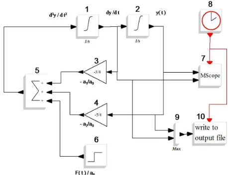
This equation can be modelled as a block diagram as shown in Fig.1.
Fig. 1: Block Diagram in XCOS to solve a general second order differential equation.
Integrating the LHS once (block 1) gives us dy/dt and integrating it once again (block 2) gives us y(t). The first derivative and y are given as initial conditions and are fed in the integration blocks 1 and 2, by clicking on them and entering in the window that appears (NOTE that the integrators have upper and lower limits. Do not forget to increase these limits for the first runs). Adding up all the terms on the RHS gives us LHS at time t=0 and integrating it twice gives us the terms v(t) and y(t) on the LHS at next time instance t = t1, which can be again fed back after proper multiplications (blocks 3 and 4)
and adding (block 5) them to obtain d2y/dt2 as input to the first integration block and the process continues till the required time of integration. The Final integration time can be set in the SetBlock properties window by going to simulate button in main menu and choosing Setup.
95 this has nothing to do with solution accuracy, it only sets the output step. The MScope (MScope, block 7), has its input ports sizes = 1 1, one for each input. The Ymin and Ymax values can be set after a test run. The refresh-period is the same as the final integrating time. As an option, the quantities are also collected into a table with the mux (block 9) and written to an output file (block 10).
2.2 Construction of Block Diagram in Xcos:
The following procedure would help to make the block diagram in Xcos. Xcos is an application of Scilab. So, start Scilab from the start program menu.
1. Click on application in menu bar and choose Xcos. It will open two windows, one is edit window and the other is pallet browser.
2. In the pallet browser, we see many blocks, such as continuous time systems, Mathematical operations, sources, sinks etc in it. Clicking on any of these shows up various blocks present in it.
3. The integration block is available in continuous time systems, the gain, summation blocks are available in mathematical operations.
4. The clock and GENSIN_f block that generates sine wave are available in sources window
5. The Mscope and write to output file blocks are in sinks window. Mux is under commonly used Blocks pallet. 6. Click and drag the required blocks on to the edit window
7. The blocks can be flipped by right clicking on them and choosing flip option 8. Left click on various blocks, to set their parameters
9. For example, left click on summation block and change the -1 to 1 and put a semicolon followed by another 1 to increase its input number to three.
10. Connect the blocks by clicking the mouse on the edge of the block at the output end and at the back of the arrow (and not at the tip of the arrow) and drag to see a line appearing. Connect it as input to the other block by leaving the mouse button at its input edge similarly.
The block diagram is ready and can be saved. Model based simulation not only helps in solving physics problems and thereby learning the underlying concepts but also helps in developing a modular approach to building and studying a model, a much needed skill. This method is used here to build the model for forced oscillator.
The forced oscillator chosen here is a simple oscillator which is subject to damping and is driven by a periodic force that is simple harmonic in nature. Its equation of motion is given by
¨
x + µ
x
˙
+ ω
02x = F
0sin
(
ωt
)
(3)
where ω0 is frequency of the simple harmonic oscillator, µ is the damping force per unit velocity per unit mass, F0 is the
amplitude of the driving force per unit mass and ω is the driving frequency in radians/second. The problem can be built step by step by starting with simulation of a simple harmonic oscillator and then adding damping coefficient to understand damped harmonic oscillator and finally bringing in the periodic driving force to implement the forced oscillator and study the resonance curve by varying the driving frequency for a certain damping coefficient. The experiment could then be repeated for a different µ to understand the effect of µ on sharpness of resonance. So, the students are initiated to the process of simulation using the simple harmonic oscillator and then are encouraged to build the damped harmonic oscillator and are finally allowed to explore the forced oscillator where in they vary the parameters in a controlled fashion. That is, they would vary the frequency by keeping the damping coefficient constant and then repeat the process for a different damping constant. This would enable them to explain the concepts of resonance and analyse how the quality of resonance changes with damping coefficient.
3. Results and Discussion:
3.1 Simple Harmonic Oscillator:
96
¨ x+ω0
2
x=0 (4)
The analytical solution for the above differential equation is x = A sin(ω0 t + φ), where A is the amplitude of
oscillation, ω0 = 2πf is the angular frequency of the oscillator in radians per second, f is the frequency in Hz and φ is the
initial phase. The Xcos model for this equation is realised as in Fig.2.
The value for frequency f is chosen as 1 Hz. The initial position is fed as 2 units in the second integrator block and the initial velocity is chosen as 0 units. The default values are zero and hence the first integrator block properties are retained. The position and velocity are fed as inputs to Mscope. Set the total integration time as 5 seconds and the refresh period in Mscope also as 5 seconds. On running the simulation, one obtains graphs which are not properly scaled. This is because, we have
Fig. 2: XCOS model for Simple Harmonic Oscillator
not set the ymin and ymax values in Mscope appropriately. Remember the initial position is set as 2 units and therefore the ymin and ymax values for ch1 in Mscope where the position is fed as input has to be changed to -2 and 2 respectively. Similarly, the amplitude of velocity will be 2 times ω0 which is going to be around 12 and hence set the ymin and ymax
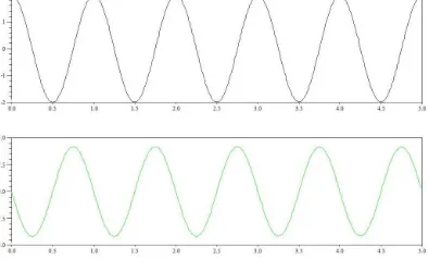
for ch2 where velocity is fed as input to -15 and 15 respectively. Then, run the simulation to obtain the graph as in Fig.3.
Fig. 3: 'x vs t' (above) and 'v vst' graphs for SHO
97
3.2 Damped Harmonic Oscillator
The simple harmonic oscillator is an idealisation and can not be achieved in the real world, for there are always forces that dampen the motion and eventually the oscillations die down and the oscillator comes to rest. So, we need to model the damping forces into the equations of motion. Here, we assume that the damping forces are proportional to velocity and the damping coefficient µ is damping force per unit mass per unit velocity.
¨
x + µ
x+ ω
˙
02x = 0
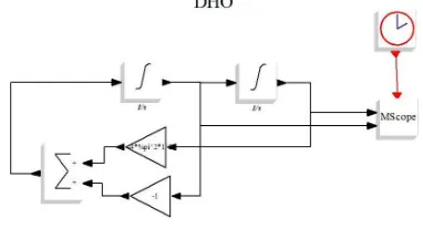
(5)The analytical solution for the above differential equation is x = x = A exp(-µt)sin(ω0 t + φ). The Xcos model for this
equation is realised as in Fig.4.
Fig. 4: XCOS model for DHO
The value for µ is chosen as -1 and the rest of the conditions are as in the previous case, except the refresh period in Mscope is changed to 10 secs and so is the total integration time in Setup. On running the simulation, under damped oscillations are obtained and this is shown in Fig.5. The students are asked to vary the value of µ and should be able to study the cases of critical and over damping by reviewing their theoretical literature. Now, they are ready to explore the forced oscillator. They could be provided with some tips as to how to add the force function in xcos and what are the parameters that can be changed in it. They can then be instructed to open the data saved in a file for analysis in Scilab and then can be asked to study the forced oscillator on their own.
Fig. 5: 'x vs t' and 'v vs t' graphs for DHO.
3.3 Forced Harmonic Oscillator
98 consider a periodic sinusoidal force as the driving force for the oscillator. The equation of motion gets modified as follows:
¨
x + µ
x
˙
+ ω
02x = F
0sin
(
ωt
)
(6)
where F0 is the amplitude of the driving force and ω is the frequency of the driving force. This can be realised in Xcos as
shown in Fig.6.
Fig. 6: XCOS model for Forced Oscillator
The number of input ports in summation block can be increased by adding a 1 followed by a semicolon in its set block properties which can be obtained by left click on the block. One can set the frequency of the sinusoid generator to be close to the natural frequency of the oscillator ω0 or one can choose it to be close to the resonance frequency sqrt{(ω02 - 2µ2).
The final integration time needs to be increased to atleast about 100 secs so that we can observe both the transient and the steady state phenomenon. The value of µ can be chosen to be 0.1 so that the damping is not too large, to start with. The ymin and ymax settings need to be adjusted accordingly by observation. The output would look as in Fig.7.
Fig. 7: Build up of resonance for frequency very close to resonance frequency
The simulation experiment here after involves varying the driving frequency about the resonance frequency and obtaining the amplitude at each of the driving frequency. The position vs time information is saved in a file by using the write to output file block. The students can be shown as to how to open the file in scilab window and perform required analysis by using the following procedure:
1. first change path giving the command cd c:\users
2. u=mopen('filename.txt','r'); (u is a file handle for filename.txt)
3. f=mfscanf(-1,u,'%e %e');\\this reads the contents of file into f; -1 option is for reading upto end of file. 4. plot(f(:,1),f(:,2)) (produces the output x vs t. f(:,1) reads the data from the first column in f.)
99 This procedure can be repeated for various files and the amplitude can be obtained for the corresponding frequencies. Finally, a plot of amplitude vs driving frequency gives us the resonance curve. The experiment can be performed by different students for different values of µ and then students can present their results to understand the impact of damping coefficient on the sharpness of resonance. A plot of resonance curve for two different values of µ is shown in Fig.8.
Fig: 8: Resonance curves for two different values of µ
4. Conclusions:
We have seen how to use model based simulation in a constructivist perspective to perform simulation of forced oscillator in a step by step process. We can conclude that Model based simulation could be an effective tool for making learning an active and social process. The students may also end up varying the amplitude of the forcing frequency and may come across chaotic systems which would encourage them to pick up material on chaos. Alternatively, if they are inquisitive enough and read their theoretical material well, they might come up with the phase vs frequency plot. May be even explain velocity resonance. This learning could be self evaluated by students by taking up simulation of other systems such as coupled oscillator or a double mass system such as double pendulum or double mass spring system. The possibilities are endless and therefore one can conclude that model based simulation is a wonderful and effective way to learning physics by doing.
Acknowledgements
The author would like to thank Mr. M.R.Ganesh Kumar for introducing Scilab and Dr Arbind Jha for introducing the ideas of constructivism.
Acknowledgments
Insert acknowledgment, if any. Sponsor and financial support acknowledgments are also placed here.
References
[1] Takwale, R. G., and P. S. Puranik. “Introduction to classical mechanics”, Tata McGraw-Hill Education, 1979.
[2] Chapra, S. C. and Canale, R. P., "Numerical Methods for Engineering", Fourth Edition, Mc Graw Hill, New York, 2002.
[3] Cavallo, Alberto, Roberto Setola, and Francesco Vasca. “Using MATLAB, SIMULINK and Control System Toolbox: a practice approach”, Prentice-Hall, Inc., 1996.
[4]Campbell, Stephen L., Jean-Philippe Chancelier, and Ramine Nikoukhah. “Modeling and Simulation in SCILAB”, Springer New York, 2006.
100
[6]Kuhlthau, Carol, Leslie Maniotes, and ANN CASPARI. “Guided inquiry: Learning in the 21st century” Greenwood Publishing Group, 2007.