DNA polymorphism in a subdivided population: the expected number of segregating sites in the two-subpopulation model.

(1)

Copyright 0 1989 by the Genetics Society of America

DNA Polymorphism in a Subdivided Population: The Expected Number

of

Segregating Sites in the Two-Subpopulation Model

Fumio Tajima

Department of Biology, Kyushu University, Hakozaki, Fukuoka 812, Japan

Manuscript received March 29, 1989

Accepted for publication June 3, 1989

ABSTRACT

Using the two subpopulation model, the expected numbers of segregating sites in a number of DNA sequences randomly sampled from a subdivided population were examined for several types of population subdivisions. It is shown that, in the case where the pattern of migration is symmetrical such as the finite island model, the expected number of segregating sites is independent of the migration rate when two or three DNA sequences are randomly sampled from the same subpopulation, but depends on the migration rate when more than three DNA sequences are sampled. It is also shown that the population subdivision can increase the amount of DNA polymorphism even in a subpopulation in some cases.

T

HE amount of DNA polymorphism in a popula-

tion can be measured by the average number of

(pairwise) nucleotide differences or the number of

segregating sites in a sample. Although their statistical

properties are already known, they have been ob-

tained under the assumption of random mating pop-

ulation (WATTERSON 1975; TAJIMA 1983). Natural

populations, however, are often subdivided into a

number of subpopulations. LI (1976) has studied the

distribution of nucleotide differences between two

randomly chosen DNA sequences in a subdivided

population by using the finite island model (MARU-

YAMA 1970; LATTER 1973; NEI 1975). Although his results give useful information on DNA polymor-

phism in a subdivided population, it is not clear

whether or not they can be applied to the case where more than two DNA sequences are sampled from the population.

In this paper I shall examine the expected number

of segregating sites in a number of DNA sequences

randomly sampled from a subdivided population by

using the two subpopulation model (NEI and FELDMAN

1972; LI and NEI 1975, 1977). Although one of the main reasons, why the two subpopulation model is

used instead of the other models such as the infinite

island model (WRIGHT 1931), the finite island model

and the stepping stone model (KIMURA and WEISS

1964; WEISS and KIMURA 1965; MARUYAMA 1969,

1977), is its simplicity, this model has the advantage of being flexible, as will be shown later.

MODEL

In this paper we assume that a population is subdi-

vided into two subpopulations, say, subpopulations 1

and 2. We denote the effective sizes of subpopulations

Genetics 123: 229-240 (September, 1989)

1 and 2 by N1 and N2, respectively. We also denote

the probability that a DNA sequence in subpopulation

1 comes from subpopulation 2 in the immediately

previous generation by m l , and the probability that a

DNA sequence in subpopulation 2 comes from sub-

population 1 in the immediately previous generation

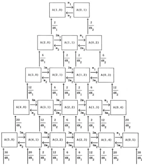
by m2. T h e scheme of this model is shown in Figure 1.

We denote by tr the mutation rate per DNA se-

quence per generation, and assume that the number

of nucleotide sites on a DNA sequence is so large that

a newly arisen mutation takes place at a site different

from the sites where the previous mutations have

occurred [the infinite site model (KIMURA 1969)]. We

also assume that the mutants are selectively neutral

[the neutral mutation model (KIMURA 1968, 1983)l.

Finally, we assume that m l , m2, l/N1 and 1/N2 are so

small that their higher order terms can be ignored.

THEORY

In this paper we use the genealogical relationship

of DNA sequences (GRIFFITHS 1980; KINGMAN 1982;

HUDSON 1983; TAJIMA 1983). Let A(i, j ) be the state

that i a n d j DNA sequences are randomly chosen from

subpopulations 1 and 2, respectively.

When one DNA sequence is randomly chosen from the population, there are two states, namely the state

that the DNA sequence is chosen from subpopulation

1 and the state that the DNA sequence is randomly

chosen from subpopulation 2. According to the defi-

nition, the former is denoted by A( 1 , 0) and the latter by A(0, 1). T h e probability that a DNA sequence in

subpopulation 1 comes from subpopulation 2 in the

immediately previous generation is ml. In terms of

(2)

S a h p o p u I a t i o t 8 I

r d

. - T I

S u b p o p u l a t i o n 2

-

N 2

E f f e c t i v e s i r e o f s u b p o p u l a t i o n

FIGURE 1 ."Scheme of the two subpopulation model used.

probability that A ( l , 0 ) changes to A(0, 1) in one generation is m l . In the same way, the probability that

A(0, 1) changes to A ( l , 0 ) in one generation is m2.

These events are shown in Figure

2.

I t should be kept

in mind that we are going back to the past.

When two DNA sequences are randomly chosen

from the population, there are three states, namely

A(2, 0), A( 1 , 1) and A(0, 2). T h e probability that one

of two DNA sequences in subpopulation 1 comes from

subpopulation 2 in the immediately previous genera-

tion is 2 m l ( l

-

m l )

=

2 m l . Therefore, the probability that A(2, 0 ) changes to A ( l , 1 ) in one generation is

2 m l . In the same way, the probability that A(0, 2)

changes to A( 1 , 1) in one generation is 2m2 approximately, and the probability that A ( l , 1 ) changes to

A(2, 0 ) or A ( 0 , 2 ) in one generation is approximately

m2 or m l , respectively.

Let us now consider the effect of random genetic drift on the change of state. T h e probability that two

DNA sequences in subpopulation 1 are derived from

a common ancestral DNA sequence in the immedi-

ately previous generation is 2/(4N1), so that the probability that A(2,O) changes to A ( 1 , 0 ) in one generation is 2/(4N1). Similarly, the probability that A ( 0 , 2 )

changes to A(0, 1) in one generation is 2/(4N2). These

events are also shown in Figure 2.

In the same way, we can obtain the necessary prob-

i(i

-

1 ) / 4 N I (3)

Prob(A(i, j ) to A(i, j

-

1)

in one generation) = j ( j

-

1)/4N2. (4)

For the derivations of (3) and (4), see HUDSON (1983)

or TAJIMA (1983). In the formulations of ( 1 ) and ( 2 )

FIGURE Z.-Flowchart of the state, A ( i j ) , that i and j DNA

sequences are randomly chosen from subpopulations 1 and 2, respectively.

the higher order terms of m1 and m2 were ignored.

This also means that each state can change only to the

adjacent states. Figure 2 shows these probabilities

when the number of DNA sequences is smaller than

six. We should again keep in mind that we are going back to the past.

Let us now obtain the expected number of segregating sites in a sample. Let S ( i , j ) be the expected

number of segregating sites in a sample of n DNA

sequences among which i DNA sequences are sampled

from subpopulation 1 and j ( = n

-

i) DNA sequences

from subpopulation

2.

Under the infinite site model,

this number is equal to the expected number of mutations which take place while A(i, j ) changes to A( 1,

0 ) or A(0, 1). First, we notice that the expected num-

ber of generations, during which A(i, j ) remains the same, is equal to the reciprocal of the probability that

A(i, j ) changes to the other states in one generation. Using (1)-(4), this probability is given by

i(i

-

1 ) + jo'

-

1)

B

= iml

+

jm2

+

-

4N1 4N2 9 ( 5 )

so that the expected number of generations is 1/B.

Since on the average nv mutations take place in each

generation, the expected number of mutations oc-

curred while A(i, j ) remains the same is given by

C = nv/B

(6) . .

-

nM1M2

(3)

DNA Polymorphism in Subpopulations

where MI = 4Nlv, M2 = 4NzV, Q1 = 4Nlml and Q 2 = S(1, 1)

23 1

4N2m2.

When A(i, j) changes, it changes to one of four

-

1). These probabilities can be obtained

from (1)-(4). That is, the probability that A(i, j)

-

1)/(4NlB) and that of A(i, j

-

1) is j ( j

-

l)/ (4N2B). Therefore, S ( i , j ) can be given by

S ( i , j ) = C + - S ( i - im 1 l , j + 1) B

j m 2

+-S(i+ 1 , j - l)+-S(i-

i(i-

1) 1 , j )

bvM2

Qz(1

+

@)M1

+

QI(1

+

~ M I M z

+

2M1[S(1, 1)

+

@S(2, l)]

and

-

+

QIMZS(0, 3)

-

2(1

+

@)M1

+

QlM2

, (10)

bq =

i[(i

-

1)S(i

-

1, j)

+

@S(i

-

1, j

+

l)].

Incidentally,

(7)

computations of S ( i , j ) , however, are straightforward although they are not always easy.

For example, when n = 2, from

(7)

we have

M1

+

QlS(1, 1) 1

+

Q1

S(2, 0) =

S(1, 1) =

S(0, 2) =

9

2M1M2

+

@M1S(2, 0)

+

QIMZS(O~ 2), (8)

QZMI

+

Q1M2

M2

+

@S(1, 1)

1

+

Q2 ,

which are equivalent to equations (9) in STROBECK

(1 987) and equations (1 3) in SLATKIN (1 987). Solving (8), we have

S(2, 0)

-

@U

+ @)M:

+

Ql(3

+

2QZ)MIMZ

+

@M;

@(l

+

Q2)MI

+

Ql(1

+

Q1)MZ

Since S(2, 0), S(1, 1) and S(0, 2) are already known, we can solve (1 0). Practically, however, it is not easy to obtain the solution of (1 0). If we use a computer, we can avoid such a difficulty. Especially, we can easily obtain the solution of (1 0) if the software for solving simultaneous linear equations is available. In the case where such a program package is not available, we can solve (10) by using (10) repeatedly. That is, we first substitute arbitrary values of S ( 3 , 0), S(2, l), S(1,

2) and S(0, 3) into (10). Then we obtain new values

of S ( 3 , 0), S(2, l), S(1, 2) and S(0, 3). We again

substitute these values into (lo), then obtain new

values. Repeating this process many times, we finally obtain the true values of S ( 3 , 0), S(2, l ) , S(1, 2) and S(0, 3). T h e number of iterations required depends

on the values of Q1 and Q, and the accuracy we seek.

In general, many iterations are required for large

values of Q1 and Q2.

In the case where n is larger than 3, we can obtain

the values of S(n, 0), S(n

-

1 , l),

. . .

and S(0, n) from S(n

-

1, 0), S(n

-

2, l),

.

. .

and S(0, n

-

1 ) by using

(7).

In this case we need the software for solving

simultaneous linear equations, or we can use the same

iteration method as mentioned in the case of n = 3.

At any rate we can obtain those values for n = 4 from

(4)

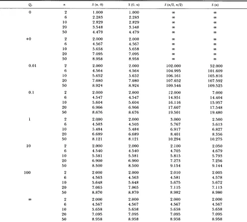
TABLE 1

Expected number of segregating sites in the case of M , = = 1 and Q =

+O 0.01 0.1 1 10 100 m

0 2

6 10 20 50 2 6 10 20 50 2 6 10 20 50 2 6 10 20 50 2 6 10 20 50 2 6 10 20 50 2 6 10 20 50 2 6 10 20 5 0

1

.ooo

2.283 2.829 3.548 4.479 2.000 4.567 5.658 7.095 8.958 2.000 4.564 5.652 7.080 8.924 2.000 4.547 5.604 6.966 8.676 2.400 4.503 5.484 6.689 8.121 2.000 4.540 5.581 6.900 8.500 2.000 4.563 5.648 7.065 8.870 2.000 4.567 5.658 7.095 8.958

1

.ooo

2.283 2.829 3.548 4.479 2.000 4.567 5.658 7.095 8.958 2.000 4.564 5.652 7.080 8.924 2.000 4.547 5.604 6.966 8.676 2.000 4.503 5.484 6.689 8.121 2.000 4.540 5.581 6.900 8.500 2.000 4.563 5.648 7.065 8.870 2.000 4.567 5.658 7.095 8.958 m m m m m m m m m m 102.000 104.995 106.161 107.652 109.546 12.000 14.951 16.1 16 17.607 19.501 3.000 5.767 6.91 7 8.401 10.294 2.100 4.705 5.815 7.273 9.154 2.010 4.581 5.675 7.115 8.982 2.000 4.567 5.658 7.095 8.958 m m m m m m m m m m 52.000 101.609 105.816 107.592 109.525 7.000 14.404 15.957 17.548 19.480 2.500 5.613 6.827 8.356 10.275 2.050 4.679 5.793 7.256 9.144 2.005 4.578 5.672 7.113 8.980 2.000 4.567 5.658 7.095 8.958

+O means that Q1 is close to 0, but not 0.

from those of n = 4. In this way we can obtain the values of S(n, 0), S(n

-

1, l),

. . .

and S(0, n ) for any

n.

Let us next consider the case where n DNA se-

quences are randomly sampled from the entire population. Let S ( n ) be the expected number of segregat-

ing sites in n DNA sequences randomly sampled from

the entire population. T h e probability that i and

n

-

i DNA sequences are randomly chosen from

subpopulations 1 and 2, respectively, given that n

DNA sequences are randomly chosen from the entire

population, is given by

n ! N’;N;-:

P(i, n

-

;‘

-

“

’’

S(n) = P(i, n

-

i ) S ( i , n

-

i). (12)

(5)

DNA Polymorphism in Subpopulations 233

M 1 = M 2 = 1 , Q1 = Q 2

2 o

.

j

-.

[

l 6 1 2

1.

S ( i . 5 0 - i )

8

l 5

m

M I = 0 . 1 . M 2 = 1 . 9, Q , = Q 2

1 2

1

S ( i . 5 0 - i )

1 t

0 1 I

c

5 0 4 0 3 0 2 0 1 0 0

1

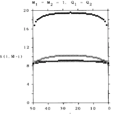
FIGURE 3.-Expected number, S ( i , 50

-

i ) , of segregating sites in a sample of 50 DNA sequences among which i DNA sequences are sampled from subpopulation 1 and 50

-

i DNA sequences from subpopulation 2. M I = M Z = 1 and QI = Qz are assumed. 0, QI =

0.1; 0, QI = 1 ; +, Q1 = 10; 0, Q1 = m.

NUMERICAL COMPUTATIONS

Let us now examine the effect of population subdivision or migration on the number of segregating sites in a sample by using the method developed in

the foregoing section. Here we will consider the six

cases.

(a) N1 = N z , m l = m2.

First we consider the case where the sizes of two subpopulations are the same and the migration rate

from subpopulation

2

to subpopulation 1 is the same

as that from subpopulation 1 to subpopulation

2.

In

this case M1 = M z and Q1 = Q2. This is a special case of the finite island model. Table 1 gives the values of

S(n, 0), S ( 0 , n), S ( n / 2 , n / 2 ) and S(n) in this case. In this table +O means that Ql or ml is close to 0, but not

0. From this table, we can see that, in the case where

two DNA sequences are sampled from the same subpopulation, the expected number of segregating sites

[S(2, 0) or S ( 0 ,

2)]

is the same as long as the migration

rate is not 0. This is consistent with the results obtained by LI (1 976) using the finite island model. That

is, the expected number of nucleotide differences

between the two DNA sequences randomly sampled

from the same subpopulation is independent of the migration rate unless the migration rate is 0. This is also true in the case where three DNA sequences are sampled, namely S(3, 0) = S ( 0 , 3) = 3 for Q1 =

Q2

>

0. When the sample size is more than three, however, the expected number of segregating sites in a sample depends on the migration rate. Table 1 shows that

S(n, 0) or S ( 0 , n) takes the smallest value when m l is 1, and that the value of S(n, 0) or S ( 0 , n) obtained by approaching m l to 0 is the same as that for the infi-

5 0 4 0 3 0 2 0 I O o

1

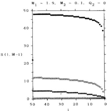
FIGURE 4.-Expected number, S ( i , 50 - i ) , of segregating sites in a sample of 50 DNA sequences among which i DNA sequences are sampled from subpopulation 1 and 50

-

i DNA sequences from subpopulation 2. M I = 0.1, M2 = 1.9 and QI = Q 2 are assumed. 0 ,

Q, = 0.1; 0, Q1 = 1; +, Ql = 10; 0, Q, = m.

nitely large value of ml. T h e values of S ( n / 2 , n/2) and

S(n) decrease as the migration rate increases, as ex-

pected. Figure 3 shows S ( i , j ) when n = 50. From this

figure, we can see the effect of migration on the value

of S(i, j ) .

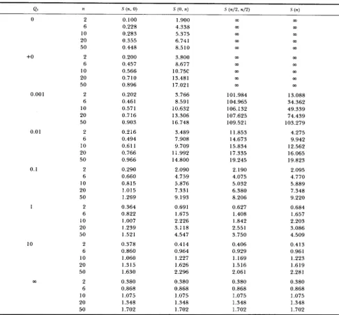
(b) N 1

<

N z , QI = Q2.

Next, we consider the case where the sizes of two subpopulations are different and the number of indi-

viduals which migrate from subpopulation 1 to sub-

population 2 is the same as that from subpopulation

2 to subpopulation 1. Table

2

shows the case where

M1 = 0.1 and M2 = 1.9. First, we notice that, as the

migration rate increases, the expected number of

segregating sites approaches the number of segregating sites expected under the random mating population with size N 1

+

N2. Next, we notice that, as the

migration rate decreases, S(n, 0) decreases but S ( 0 , n)

increases. T h e latter property is important, since the expected number of segregating sites [ S ( O , n)] in n

DNA sequences sampled from the large subpopula-

tion is larger than that of random mating population with size N1

+

N2. Figure 4 also shows the effect of

migration on the expected number of segregating sites

in a sample.

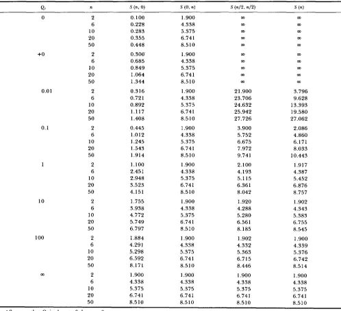
(c) N 1

<

N 2 , ml = m2.

Here, we examine the case where the sizes of two

subpopulations are different and the proportion of

immigrants in each subpopulation is the same in every

generation. Table 3 shows the case where MI = 0.1,

(6)

M I - 0 . 1. M 2 - 1. 9 , Q 2 = 1 9 Q ,

1 5

S ( i . 5 0 - i )

1 0

5

0 -I I

5 0 4 0 3 0 2 0 1 0 0

1

FIGURE 5.-Expected number, S ( i , 50

-

i), of segregating sites in a sample of 50 DNA sequences among which i DNA sequences are sampled from subpopulation 1 and 50

-

i DNA sequences from subpopulation 2. MI = 0.1, MP = 1.9 and Q:! = 19Q are assumed.

A , Q 1 = O . O l ; O , Q I = O . l ; O , Q 1 = l ; O , Q l = ~ .

MI ~ 0 . 1. M 2 = 1. 9 . Q 2 ~ 0

l 5

-

l 2

i

t

5 0 4 0 3 0 2 0 1 0 0

I

FIGURE 6.-Expected number, S ( i , 50 - i), of segregating sites in a sample of 50 DNA sequences among which i DNA sequences are sampled from subpopulation 1 and 50

-

i DNA sequences from subpopulation 2. M I = 0.1, MP = 1.9 and Q2 = 0 are assumed. 0 ,

41 = 0.1; 0,

el

= 1 ; +, Q1 = 10; 0, = m.

sites in n DNA sequences randomly sampled from the

same subpopulation approaches that of random mating population with size ~ N I N ~ / ( N ~

+

N2).

Large values of S ( 0 , n) are also observed in the case of small

is also shown in Figure 5 .

(d) N 1

<

N P , m2 = 0.

In this and the following cases we assume that the migration takes place only in one direction, namely

from subpopulation 2 to subpopulation 1. Therefore,

the expected number of segregating sites in DNA

sequences randomly sampled from subpopulation 2 is

1 8

S ( i . 5 0 - i )

1 2

6

0

5 0 4 0 3 0 2 0 1 0 0

1

FIGURE 7,"Expected number, S ( i , 50 - i), of segregating sites in a sample of 50 DNA sequences among which i DNA sequences are sampled from subpopulation 1 and 50

-

i DNA sequences from subpopulation 2. M I = M2 = 1 and 42 = 0 are assumed. 0 , Q1 =

0.1; 0, Q1 = 1 ; +, QI = 10; 0, QI = m.

M I - 1. 9 . M 2 = 0 . 1 . Q 2 = 0

5 0 4 4

I

-.

i

0

5 0 4 0 3 0 2 0 1 0 0

1

FIGURE 8.-Expected number, S(i, 50 - i), of segregating sites

in a sample of 50 DNA sequences among which i DNA sequences are sampled from subpopulation 1 and 50

-

i DNA sequences from subpopulation 2. MI = 1.9, M:! = 0.1 and

42

= 0 are assumed. 0,

Ql = 0.1; 0, Q1 = 1; +, Q I = 10; 0 , Q , = m.

independent of the rate of migration from subpopu-

lation

2

to subpopulation 1. Table

4

shows the case

where M , = 0.1 and MP = 1.9. As expected, the

expected number of segregating sites in DNA se-

quences randomly sampled from subpopulation 1 in-

creases as the migration rate increases, and reaches

the same value as that of subpopulation 2. Figure 6 also shows the effect of migration on the expected number of segregating sites.

(e) N 1 = N P , m2 = 0.

Table 5 shows the case where MI = M P = 1 and

4

2

(7)

DNA Polymorphism in Subpopulations 235

TABLE 2

Expected number of segregating sites in the case of M , = 0.1, M 2 = 1.9 and =

41 n S (n, 0) S (0, n) S ( 4 2 , n I 2 ) s ( 4

0 2 0.100 1.900 m

6 0.228 4.338 m

10 0.283 5.375 m m

20 0.355 6.741 m

50 0.448 8.510 m

m

03

m

+O

0.01

0.1

1

10

100

m

2 0.290 2.090

6 0.662 4.772

10 0.820 5.913

20 1.029 7.415

50 1.299 9.362

m m m m m

m

2 0.307 2.089 2 1

.ooo

3.881

6 0.700 4.770 22.926 9.747

10 0.867 5.909 23.878 13.421

20 1.086 7.409 25.208 19.361

2 0.445 2.082 3.900 2.250

10 1.245 5.881 6.831 6.557

20 1.544 7.366 8.163 8.409

2 1.145 2.045 2.190 2.057

6 2.552 4.666 4.401 4.697

10 3.070 5.775 5.366 5.821

20 3.670 7.228 6.663 7.300

50 4.325 9.096 8.397 9.208

2 1.845 2.008 2.019 2.009

6 4.137 4.585 4.509 4.587

10 5.008 5.680 5.547 5.683

20 6.024 7.121 6.880 7.126

50 7.108 8.984 8.561 8.996

2 1.983 2.001 2.002 2.001

6 4.516 4.569 4.560 4.569

10 5.574 5.660 5.644 5.661

20 6.931 7.098 7.063 7.099

50 8.583 8.961 8.876 8.962

50 1.368 9.351 27.005 26.472

6 1.012 4.751 5.873 5.208

50 1.917 9.282 9.960 10.738

2 2.000 2.000 2.000 2.000

6 4.567 4.567 4.567 4.567

10 5.658 5.658 5.658 5.658

20 7.095 7.095 7.095 7.095

50 8.958 8.958 8.958 8.958

+O means that Ql is close to 0, but not 0.

segregating sites in DNA sequences randomly sampled

from subpopulation 1 decreases as the migration rate

increases. Large values of S ( n , 0) are observed when

the migration rate is small. T h e effect of migration

on S ( i , j ) is also shown in Figure

7.

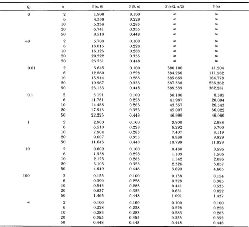
( f ) N I

>

NP, m2 = 0.

Here we examine the case where the migration takes place only in the direction from a small subpopulation to a large subpopulation. This is an unusual case, so that this type of migration is very rare in nature, if any. Table 6 shows the case where M I =

1.9, M2 = 0.1 and Q 2 = 0. Extremely large values of

S(n, 0) are observed when the migration rate is small.

Figure 8 also shows the relationship between the

migration rate and the expected number of segregating sites in a sample.

CONCLUSION AND DISCUSSION

In this paper we have examined the effect of pop-

ulation subdivision or migration on the expected num-

ber of segregating sites in a sample by using the two subpopulation model, and obtained the following results: (1) T h e expected number of segregating sites in

(8)

+O

0.001

0.0 1

0.1

1

10

m

TABLE 3

Expected number of segregating sites in the case of M , = 0.1, M 2 = 1.9 and = 19@

QI n S (n, 0) S (0, n) S (n/2,n/2) S (n)

0 2 0.100 1.900 m m

6 10

m

20

m

50 0.448 8.510 m m

m

2 0.200 3.800 m

6 0.457 8.677 m

m

10

m

0.566 10.750 m

20 0.710 m m

m

13.48 1

50 0.896 17.021 m m

0.228 4.338 0.283 5.375

0.355

m m

6.741 m

2 0.202 3.766 101.984 13.088

6 0.461 8.591 104.965 34.362

10 0.571 10.632 106.132 49.339

20 0.716 13.306 107.625 74.439

50 0.903 16.748 109.521 103.279

2 0.2 16 3.489 11.853 4.275

6 0.494 7.908 14.673 9.942

10 0.61 1 9.709 15.834 12.562

20 0.766 1 1.992 17.335 16.065

50 0.966 14.800 19.245 19.823

2 0.290 2.090 2.190 2.095

6 0.660 4.759 4.075 4.770

10 0.815 5.876 5.032 5.889

20 1.015 7.331 6.380 7.348

50 1.269 9.193 8.206 9.220

2 0.364 0.691 0.627 0.684

6 0.822 1.675 1.408 1.657

10 1.007 2.226 1.842 2.203

20 1.239 3.1 18 2.551 3.086

50 1.521 4.547 3.750 4.509

2 0.378 0.414 0.406 0.41 3

6 0.860 0.964 0.929 0.961

10 1.060 1.227 1.169 1.223

20 1.315 1.626 1.516 1.619

50 1.630 2.296 2.061 2.281

2 0.380 0.380 0.380 0.380

6 0.868 0.868 0.868 0.868

10 1.075 1.075 1.075 1.075

20 1.348 1.348 1.348 1.348

50 1.702 1.702 1.702 1.702

+O means that Q1 is close to 0, but not 0.

subpopulation generally depends on the migration

rate. T h e expected number of segregating sites in the two DNA sequences randomly sampled from the same subpopulation, however, is independent of the migration rate when the pattern of migration is symmetrical such as the finite island model or case (a). This is also

true when the three DNA sequences are sampled.

When the sample size is larger than three, this is not the case.

(2)

In some cases [in cases (b), (c), (e) and

(f)], the expected number of segregating sites in DNA

sequences randomly sampled from the same subpopulation can be larger than that expected from the

random mating population whose effective size is the

same as that of the entire population or the sum of

the two effective sizes of subpopulations. In other

words, the population subdivision can increase the

amount of DNA polymorphism even in a subpopula-

tion in some cases.

Recently Tajima (1989) has developed a statistical

method for testing the neutral mutation hypothesis

by using the relationship between the number of

segregating sites and the average number of (pairwise)

nucleotide differences among a sample of DNA se-

quences. This method assumes that the population

(9)

DNA Polymorphism in Subpopulations 237

TABLE 4

Expected number of segregating sites in the case of M, = 0.1, M p = 1.9 and @ = 0

0.01

0.1

1

10

100

0 2 0.100 1 .goo m m

6 0.228 4.338 m m

10 0.283 5.375 m m

20 0.355 6.741 m m

50 0.448 8.510 m m

+O 2 0.300 1 .goo m m

6 0.685 4.338 m m

10 0.849 5.375 m m

20 1.064 6.741 m m

50 1.344 8.510 m m

2 0.316 1.900 2 1.900 3.796

6 0.72 1 4.338 23.706 9.628

10 0.892 5.375 24.632 13.393

20 1.117 6.741 25.942 19.580

50 1.408 8.5 10 27.726 27.062

2 0.445 1 .goo 3.900 2.086

6 1.012 4.338 5.752 4.860

10 1.245 5.375 6.675 6.171

20 1.543 6.741 7.972 8.033

50 1.914 8.510 9.741 10.443

2 1.100 1.900 2.100 1.917

6 2.451 4.338 4.193 4.387

10 2.948 5.375 5.115 5.452

20 3.523 6.741 6.361 6.876

50 4.151 8.510 8.042 8.757

2 1.755 1.900 1.920 1.902

10 4.772 5.375 5.280 5.383

20 5.749 6.741 6.56 1 6.755

2 1.884 1 .goo 1.902 1.900

6 4.291 4.338 4.332 _4.339

5.298 5.375 5.363 5.376

50 8.171 8.510 8.446 8.514

1.900 4.338

6 3.938 4.338 4.288 4.343

50 6.797 8.510 8.185 8.545

10 20 6.592 6.741 6.715 6.742

m 2 1 .goo 1 .goo 1.900

4.338 4.338 4.338

6

10 20 6.741 6.741 6.741 50

5.375 5.375 5.375 5.375

6.741 8.510 8.510 8.510 8.510

(10)

0.01

0.1

1

10

100

0 2 1.000 1

.ooo

m

6 2.283 2.283 m

10 2.829 2.829 m

20 3.548 3.548

50 4.479

+O 2 3.000 1.000 m

m

m m

4.479 m m

6

10 20

50 13.438 4.479 m m

m

6.850 2.283 m m

8.487 2.829 m

10.643

m m

3.548 m

2 2.980 1.000 201

.ooo

101.495

10 8.418 2.829 205.153 204.614

20 10.542 3.548 206.644 206.583

6 6.800 2.283 203.987 197.507

50 13.280 4.479 208.538 208.5 17

1 1.455

6.396 2.283 23.883 23.040

10 7.867 2.829 25.040 24.858

20 9.743 3.548 26.528 26.468

50 12.070 4.479 28.421 28.399

2 2.000 1

.ooo

3.000 2.250

6 4.488 2.283 5.300 5.099

10 5.446 2.829 6.375 6.264

20 6.610 3.548 7.817 7.765

50 7.980 4.479 9.693 9.673

2 1.182 1

.ooo

1.200 1.145

6 2.757 2.283 2.719 2.687

10 3.500 2.829 3.470 3.443

20 4.541 3.548 4.584 4.562

50 5.934 4.479 6.224 6.210

2 1.020 1.000 1.020 1.015

6 2.342 2.283 2.331 2.328

10 2.924 2.829 2.905 2.902

20 3.726 3.548 3.692 3.690

50 4.862 4.479 4.809 4.806

m 2 1.000 1.000 1.000 1.000

6 2.283 2.283 2.283 2.283

10 2.829 2.829 2.829 2.829

20 3.548 3.548 3.548 3.548

50 4.479 4.479 4.479 4.479

2 2.818 1.000 2 1.000

6

(11)

DNA Polymorphism in Subpopulations 239

TABLE 6

Expected number of segregating sites in the case of M, = 1.9, M n = 0.1 and = 0

+O

0.01

0.1

1

10

100

0 2 1 .goo 0.100 m m

6 4.338 0.228 m m

10 5.338 0.283 m m

20 6.741 0.355 m m

50 8.510 0.448 m m

2 5.700 0.100 m m

6 13.015 0.228 cc m

10 16.125 0.283 cc

20 20.222 0.355 m m

50 25.531 0.448 cc m

m

2 5.645 0.100 380.100 4 1.204

6 12.880 0.228 384.266 11 1.582

10 15.944 0.283 385.669 164.778

20 19.967 0.355 387.338 256.362

50 25.153 0.448 389.339 362.281

2 5.191 0.100 38.100 8.305

6 11.781 0.228 41.987 20.094

10 14.488 0.283 43.357 26.543

20 17.943 0.355 45.007 36.022

50 22.225 0.448 46.999 46.060

2 2.900 0.100 3.900 2.988

6 6.510 0.228 6.292 6.700

10 7.904 0.283 7.407 8.1 19

20 9.607 0.355 8.888 9.829

50 1 1.645 0.448 10.799 1 1.829

2 0.609 0.100 0.480 0.596

6 1.538 0.228 1.103 1.506

10 2.125 0.283 1.542 2.086

20 3.103 0.355 2.326 3.057

50 4.649 0.448 3.690 4.605

2 0.155 0.100 0.138 0.154

10 0.543 0.283 0.441 0.535

20 0.837 0.355 0.65 1 0.822

m 2 0.100 0.100 0.100 0.100

6 0.390 0.228 0.328 0.385

50 1.465 0.448 1.091 1.437

6 0.228 0.228 0.228 0.228

10 0.283 0.283 0.283

20

0.283 0.355 0.355 0.355 0.355

50 0.448 0.448 0.448 0.448

(12)

rium unless the migration rate is very small. That is, the expected number of segregating sites in a sample is close to that expected in the random mating popu-

lation, when

Q1

is larger than 10. This means that the

migration of only a few number of individuals in every

generation is sufficient for his method to be applicable

as long as the effective population sizes stay constant. In this paper we have used the two subpopulation

model, and obtained interesting results of which some

could not be obtained from the other models. Al-

though the actual pattern of migration in natural

populations seems to be more complicated than the two subpopulation model, this model might be useful for obtaining a rough idea about the effect of population subdivision or migration on DNA polymor- phisms.

I thank two anonymous referees for useful comments on this paper.

LITERATURE CITED

GRIFFITHS, R. C., 1980 Lines of descent in the diffusion approx- imation of neutral Wright-Fisher models. Theor. Popul. Biol. 17: 37-50.

HUDSON, R. R., 1983 Testing the constant-rate neutral allele model with protein sequence data. Evolution 37: 203-217.

KIMURA, M., 1968 Evolutionary rate at the molecular level. Na- ture 217: 624-626.

KIMURA, M., 1969 The number of heterozygous nucleotide sites maintained in a finite population due to steady flux of mutations. Genetics 61: 893-903.

KIMURA, M., 1983 The Neutral Theory of Molecular Evolution.

Cambridge University Press, London.

KIMURA, M., and G. H. WEISS, 1964 The stepping stone model of population structure and the decrease of genetic correlation with distance. Genetics 4 9 561-576.

KINGMAN, J. F. C., 1982 On the genealogy of large populations. J. Appl. Probab. 19A: 27-43.

LATTER, B. D. H., 1973 T h e island model of population differ- entiation: A general solution. Genetics 73: 147-157.

LI, W.-H., 1976 Distribution of nucleotide differences between two randomly chosen cistrons in a subdivided population: the finite island model. Theor. Popul. Biol. 10: 303-308.

LI, W.-H., A N D M. NEI, 1975 Drift variances of heterozygosity and genetic distance in transient states. Genet. Res. 25: 229- 248.

LI, W.-H., and M. NEI, 1977 Persistence of common alleles in two related populations or species. Genetics 86: 901-914.

MARUYAMA, T., 1969 Genetic correlation in the stepping stone model with non-symmetrical migration rate. J. Appl. Probab. 6: 463-477.

MARUYAMA, T., 1970 Effective number of alleles in a subdivided population. Theor. Popul. Biol. 1: 273-306.

MARUYAMA, T., 1977 Stochastic Problems in Population Genetics.

Springer-Verlag, Berlin.

NEI, M., 1975 Molecular Population Genetics and Evolution. North- Holland, Amsterdam.

NEI, M., and M. W. FELDMAN, 1972 Identity of genes by descent within and between populations under mutation and migration pressures. Theor. Popul. Biol. 3: 460-465.

SLATKIN, M., 1987 The average number of sites separating DNA sequences drawn from a subdivided population. Theor. Popul. Biol. 32: 42-49.

STROBECK, C., 1987 Average number of nucleotide differences in a sample from a single subpopulation: a test for population subdivision. Genetics 117: 149-153.

TAJIMA, F., 1983 Evolutionary relationship of DNA sequences in finite populations. Genetics 105: 437-460.

TAJIMA, F., 1989 Statistical method for testing the neutral mutation hypothesis by DNA polymorphism. Genetics (in press). WATTERSON, G. A , , 1975 On the number of segregating sites in

genetic models without recombination. Theor. POPU~. Biol. 7:

256-276.

WEISS, G. H., and M. KIMURA, 1965 A mathematical analysis of

the stepping stone model of genetic correlation. J. Appl. Probab. 2: 129-149.

WRIGHT, S . , 1931 Evolution in Mendelian populations. Genetics 16: 97-159.