A NEW METHOD FOR ESTIMATING THE EFFECTIVE POPULATION SIZE FROM ALLELE FREQUENCY CHANGES

Copyright 0 1983 by the Genetics Society of America

A NEW METHOD FOR ESTIMATING THE EFFECTIVE

POPULATION SIZE FROM ALLELE FREQUENCY CHANGES

EDWARD POLLAK’

Center for Demographic and Population Genetics, University of Texas at Houston, Houston, Texas 77025

Manuscript received April 3,1981

Revised copy accepted March 23,1983

ABSTRACT

A new procedure is proposed for estimating the effective population size, given that information is available on changes in frequencies of the alleles at one or more independently segregating loci and the population is observed at two or more separate times. Approximate expressions are obtained for the variances of the new statistic, as well as others, also based on allele frequency changes, that have been discussed in the literature. This analysis indicates that the new statistic will generally have a smaller variance than the others. Esti- mates of effective population sizes and of the standard errors of the estimates are computed for data on two fly populations that have been discussed in earlier papers. In both cases, there is evidence that the effective population size is very much smaller than the minimum census size of the population.

T is well known that if the frequency of a neutral allele changes from x in one

I

generation to x ’ in the next, then E[(x’

-

x ) ~ ] = x ( 1 - x)/ZN, where N is the effective population size. This suggested to KRIMBAS and TSAKAS (1971) that, if

xi0 and xi1 are the frequencies of allele Ai at a locus at times 0 and t, N can be estimated from

1 (Xi1

-

X i 0 ) 2

K

i - 1 xidl

-

Xio)’

F a = -

where K is the number of alleles. Now the observed change in the frequency of any particular allele is partly attributable to sampling error. To adjust for the associated upward bias, these authors assumed that it is appropriate to subtract

1/2S0

+

1/2S1 from

Fa,

where SO and

SI

are the sizes of the samples observed in generations 0 and t . The resulting difference is then divided by t to allow for having t generations pass between observations, rather than just one. We are thus led to the estimator

proposed by KRIMBAS and TSAKAS (1971) and studied by LEWONTIN and KRAK-

The procedure that I have just described has recently been criticized by PAMILO and VARVIO-AHO (1980) and by NEI and TAJIMA (1981). One problem that can arise is that x i 0 may be zero and x i l positive, which would cause Fa to

become infinite. A way to bypass this difficulty, which was used by KRIMBAS

and TSAKAS (1971), is to replace x i o by x i l in the denominator of

Fa

whenever x i o

is equal to zero. This is, however, open to question, because it must necessarily complicate the sampling theory to an extent that it is difficult, if not impossible, to measure.

Another approach is to always put ( x i 0

+

x i 1 ) / 2 = jii in place of xi0 in the

denominator of

Fa.

Then the modified ratio

AUER (1973).

presented by NEI and TAJIMA (1981) as an alternative to Fa, can never be infinite. It also has the advantage that Z, has a smaller standard error than X,O.

A third statistic,

F, = - l K - XLnY

K $ = I ~1 - XLiXtn '

was also proposed by these authors. Computer simulations led them to conclude that, among

Fa,

F b and F,, Fa has the largest variance and F, the smallest.

These computer simulations, as well as those run by LEWONTIN and KRAKAUER

(1973) on Far suggest that

Fa,

Fb and F, are approximately equal to multiples of

chi-squared random variables. This suggests the feasibility of a mathematical analysis of the distribution theory of at least one of these statistics, or of a statistic that is similar to them in form. One thing that should be noted, however, is that

Fa,

Fb and F, are sums of terms having numerators that are like squared shifts in allele frequencies and denominators that are not, in general, like expected values of the frequencies before the shifts.

If, however, K = 2, it can be shown that

Fb = -

+

( x 1 1

-

xlo)2 (x21 - xzo)2 x 1 Zz

where

Z,

is an unbiased estimator of the initial frequency of A, if there is no selection. With this fact as a point of departure, it shall be shown in this paper that

(XI1

-

xlo)2 K

(PK1=

x-1 21

is a variable that is approximately a multiple of a chi-squared random variable with

K

- 1 d.f. This leads to a new statistic F K ~ that is identical with F b when K

EFFECTIVE POPULATION SIZE 533

Much of the theory in this paper is based upon a variant of the diffusion approximation that is applicable if t/N is small, so that moments of shifts in allele frequencies can be taken to be approximately equal to their initial values between times 0 and t. This theory will be in the APPENDIX, and the main results

in it will be invoked as needed in the body of the paper.

Point estimates of N and approximate standard errors of these estimates, based upon the new statistic, will be computed for data on fly populations that have been presented by KRIMBAS and TSAKAS (1971) and BEGON, KRIMBAS and

LOUKAS (1980).

UNDERLYING ASSUMPTIONS

Let us suppose that a finite population with NA individuals is observed in generations 0, tl, t z ,

. . .

, t, and that at that time ti the genetic makeup of a sample of S j individuals is recorded. Then, if there are identifiable alleles A1, Az,

.

. .

, AK at a particular locus that is being studied, the following data will be available.

Generation Sample size Sample frequency of Ai

0

so

Xi0

tl

s1

Xi1

t2 s2 Xi2

tr S r Xir

We shall consider two ways of obtaining the samples, which, following the terminology of NEI and TAJIMA (1981), shall be called sampling schemes 1 and 2. In the first scheme, which was considered by PAMILO and VARVIO-AHO (1980) and SOURDIS and KRIMBAS (1980), individuals are sampled after reproduction. This is mathematically equivalent to returning them to the population after their genotypes are examined, because, in either case, it is assumed that the sampling does not affect the effective population size. In addition, this means that the genes observed at time t j and those observed later can be assumed to be

independently chosen from the gene pool at time t,. It was also assumed by these authors, as well as by NEI and TAJIMA (1981), that NA = N, although, as we shall see, this is not a necessary part of this sampling scheme.

The second sampling scheme is based upon the model considered by SCHAF- FER, YARDLEY and ANDERSON (1977) and WILSON (1980) in their work on testing for the effects of selection on allele frequency changes. In this scheme it is

assumed that NA is much larger than N and that two samples are separately chosen from among the NA individuals in the population. The genotypes are examined in one of the samples, whereas the second is chosen to be the subpopulation of reproducing individuals.

not to use the data to test whether selection has occurred, but rather to estimate

N from the observed changes in the frequencies of A1,

.

. .

, AK.

A NEW STATISTIC FOR ESTIMATING N

If there are two alleles and r = 1, we have seen that in estimating N it is sensible to compute the statistic

1,

-[

2 El(1 - El) xz(1- E2)

1 ( X l l

-

xlo)2 +

(71

-

x20)2

where Ei = (xi0

+

Xi1)/2. Since x11

-

x10 = -(x21

-

xm) and E2 = 1

-

El, this expression is equal to

I

1 (Xll

-

Xl0l2 (x21 - xz0l2 ( X n

-

xlo)2

[

&

+

4

= 2

[

+

1 - x1 x11

+

x10 x21

+

x20

which leads immediately to the K allele generalization

The expression (PKI happens to be twice as large as a quantity mentioned by

BHATTACHARYA (1946) as a measure of the distance between two vectors of relative frequencies when these vectors do not deviate greatly from each other.

When r

>

1, we consider the generalization

a function of allele frequencies that incorporates in a simple way the pooling of data from r separate recordings of frequency changes among K alleles at a locus. Since E(xij) = E(xi,j-1) = pi, the frequency of Ai in generation 0, it follows that if Xij

-

pi dij and xi.j-1 - pi = di,j-l are small

where vij = xij - xi, j-1.

Expression (3) will now be used to obtain an approximation to E(pKr). Clearly

E(v$) = E[(xij

-

pi) - (Xi,j-l- &)I2

(4)

= V(xij)

+

V(Xi,j-I) - 2 C O V ( X i j , xi,j-l),

where V(x) denotes the variance of x.

Now under either of the sampling schemes the 2Sj genes that are chosen for observation at time t are removed without replacement from among ZNA genes while they are being observed. Therefore, the underlying distribution is hyper- geometric, so that, in particular,

EFFECTIVE POPULATION SIZE 535

scheme. Under the first sampling scheme the individuals observed at time tj 1 1 arise from a process that can be decomposed into three stages. In the first there is reproduction for tj

-

1 generations with effective population size N, whereas in the second, NA young individuals are produced. Then, in the last stage, there is hypergeometric sampling of 2Sj genes from a total of 2 N A . Thus, the population behaves as if it reproduced for t,

+

1 generations, with NA and s j ( 2 N ~

-

1)/2(N~

-

S j ) being the effective population sizes in the last two generations. Hence, it may be shown, if we imitate the reasoning employed by

CROW

and KIMURA (1970), that

This expression has been derived by NEI and TAJIMA (1981) in the special case in which NA =

N,

so that reproduction is by binomial sampling.

If we now denote the frequency of Ai in the population at time tj-1 by Pi,j-l,

C O v ( X i j 9 xi, j-1)

E[(xij

-

pij-1

+

pi,,-1

-

Pi)(Xi,j-l- Pi,j-1+ pij-1- pi)]

= E[(xij

-

pi,j-l)(xi,j-l

-

pi,j-d]

+

E[(xij- pi,j-d( pi,j-1- pi)]

+

E[( pi.j-1

-

Pi)(xi,j-1

-

pi,j-d]

+

E[(pi,j-1-

The middle two terms are equal to zero, because, with no selection, the conditional expectations of both Xij and xi,j-l, given ~ i , j - ~ , are pi,j-~. Since, under sampling scheme 1, the genes observed at times tj and tj-1 are independ- ently chosen from the population with allele frequencies pi,j-l, the first term is also equal to zero. Therefore,

pi(l

-

pi)

[

1

-

(1

-&)"'I.

(7)

because the gene pool in generation ti-1 arises from tj-1 generations of repro- duction.

If j

>

1, we may combine expressions (6) and (7) with (4) to obtain

j

>

1. If j = 1, we find, by substituting (5) to (7) in (4) that

2s0

-

2so ~ N A - 1 (9)

It now follows from (3), (8) and (9) that

Expressions (2) and (10) imply that the statistic

has an expected value satisfying

tr

-

(2r - 1)

--+

1

_{( L + L ) .}

E ( F K r ) =: 2N

~ N A j = 1 2Sj 2Sj-1

It is unfortunate that NA, which will usually be unknown in practice, appears along with N on the right side of (12). If, however, our estimation procedure is to be applied to a population with high fecundity and high mortality rates, it is reasonable to assume that N A is much larger than N, as well as S;, j = 1,

.

. .

, r.

In this case we may replace E ( F K ~ ) by F K ~ in (12) to obtain the estimator

A t, - (Zr - 1)

r / * I \ - I *

In the other extreme case, which was considered by NEI and TAJIMA (1981), we assume that NA = N. Now ~ / N A is the same size as 1/N instead of being much smaller, so that the estimator takes the form

A t,

-

2r

Nkr =

2

[

F K r - C

j:,

(215,

-+-

2 5 3 3 3 a

When r = 1, the calculations in (14) are analogous to some of those proposed by NEI and TAJIMA (1981) for sampling scheme 1. The only difference is that F K ~ is used in place of Fa or F,.

Under the second sampling scheme, expressions (4) and (5) still apply but (6)

EFFECTIVE POPULATION SIZE 537

reproduction for tj

-

1 generations with effective population size N is followed by having NA young individuals in generation t;, from which 2s; genes are chosen for the sample. Thus, if j

>

1,

since it has been assumed that NA is much larger than

N.

Because of this assumption it also follows that the samples of genes chosen for reproduction and observation at time tj-1 are approximately independently distributed. Thus, any covariance between the sample allele frequencies at times tj and t;-1 is

entirely due to their derivation in common from the population at time ti-1 - 1. Hence, it follows that

Cov(xij, xi,j-d

1 ~ ( N A -

N)]

(1

--

21JtJ-1-1}

z Pi(1 - pi)

{

1

-

[

1

--

2N Z N A - ~

z Pi(l - pi)

[

1

-

(1

-

47.

Expressions (15) and (16) are consistent with results given by SCHAFFER, YARDLEY

and

ANDERSON

(1977), WILSON (1980) and NEI and TAJIMA (1981). If we now substitute (15) and (16) in (4) we obtain

for j

>

1. If j = 1, (5) must also be substituted in (4), and thus, since the right side

of (16) is now zero, we find that

Therefore, if E(FK,) is replaced on the left side of (19) by FKrl we are led to the estimator

Once again, when r = 1, our results are analogous to those obtained by NEI and

TAJIMA (1981) for F,.

THE VARIANCES OF THE ESTIMATORS OF N

For simplicity I shall discuss only sampling scheme number 2. If it is desired to obtain analogous results for sampling scheme 1, only minor changes are necessary.

Because the variance of F K ~ is small, as is shown in the APPENDIX, it follows

from (20) that

so that

where V(FK~) is given by expression (A7) in the APPENDIX. The same analysis as

that leading to (21) may also be applied to the other statistics that have been proposed as estimators of N. The result is, in each case, an expression of the same form as (21), with N4 in the numerator, rather than N2, as claimed by

LEWONTIN and KRAKAUER (1973).

It is possible to incorporate information from L loci, rather than just one. For locus A, we have, by (ll),

where k h = KA

-

1. Now, if data are obtained from the same number of individuals for each locus, and r = 1, it is clear from (19) that k x F K A 1 has a mean

equal to

k r [ ? + - + L ] . 1 2N

zs1

2so

This suggests that we consider the weighted average

1 L

A-1

EFFECTIVE POPULATION SIZE 539

weighting the information from each locus by its number of independent allele frequencies.

In general, if it is possible to classify S j A individuals with regard to their

alleles at locus A at time t j , it follows from (19) and (23) that

h-1

Hence, we have the estimator

A-1

If there is independent assortment, expression (23) implies that

where V(FKAr) is given by (A7). Finally, expressions (24) and (25) imply that

and hence

where V(&) is given by (26).

It is clear from (27) that V(N$) can be quite large unless, perhaps, data on frequency changes are available for many genetic variants. It is also helpful to have t, as large as possible.

We conclude this section by noting some properties of the variance of F-. First, if r = 1, the second term in (A7) is replaced by 0 because it arises only if

allele frequencies are observed at three or more time points. Equivalently, (A7) applies to locus A if SO and SI are replaced by SOA and SI,,. Hence, if r = 1 and there is no selection, (26) and (A5) imply that

Second, if there happens to be the same number of individuals observed with regard to variation at each locus, it follows from (19) and (24) that the estimate simplifies further to

t ?

kx

X = 1

Third, if r 2 2, we can compute a sample estimate of the variance of

N&

by substituting the sample estimate for the true effective population size in (A14).

TWO NUMERICAL EXAMPLES

From the description of the sampling procedure in the paper of KRIMBAS and

TSAKAS (1971), it seems that sampling scheme number 2 is a more realistic model than sampling scheme number 1. Thus, all of the computations in this section shall be based upon the assumption that the former holds.

KRIMBAS and TSAKAS (1971) took samples from a population of the olive fruit fly Dacus oleae in 1966,1967 and 1968, at intervals approximately 1 yr in length. The number of generations per year was estimated by them to be four. Individ- uals were classified with respect to two highly polymorphic and unlinked loci, denoted by A and

B.

The sample sizes were SO = 474, SI = 312 and S2 = 400 for locus A and So = 469, SI = 281 and S2 = 409 for locus

B.

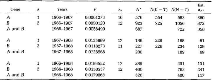
I have used their allele frequency data to compute estimates of N and of the standard errors of the estimates. These are given in Table 1. For comparison, I have also tabulated the corresponding estimates computed by KRIMBAS and TSAKAS (1971) and NEI and TAJIMA (1981). These are denoted by N(K - T) and N(N - T), respectively. The three sets of estimates are of the same order of magnitude.

One thing that is evident from this table is that the estimates of N for

1967-1968 are much smaller than those for 1966-1967. This is not surprising

because of the heavy application of insecticides in the later period. In addition, the estimates of N within a period agree reasonably well for loci A and

B.

TABLE 1

Estimates of N and of the standard errors of the estimates in the population observed by Krimbas and Tsakas

Est.

A 1 1966-1967 0.0061273 16 576 554 583 360

A and B 1966-1967 0.0056490 687 722 358

Gene A Years F k h N * N(K - T) N ( N - T) ( I N .

B 2 1966-1967 0.0050120 12 923 725 1056 872

A 1 1967-1968 0.0135889 17 186 226 168 8 1

B 2 1967-1968 0.0118273 11 227 228 234 129

A and B 1967-1968 0.0128968 200 189 69

A 1 1966-1968 0.0193552 17 289 291 131

B 2 1966-1968 0.0158537 12 400 762 241

EFFECTIVE POPULATION SIZE 541

The computed standard errors of the estimates of N are of the same order of magnitude as the estimates themselves. Thus, the number N4 in the numerators

of (21) and (27) are, to some extent, counterbalanced by the squares of kl, k2 or

kl

+

kg, which appear in the denominator of (26). KRIMBAS and TSAKAS (1971) estimate that the minimum population size was 4000 in the period during which the population was observed. The evidence is, thus, strong that the effective population size was very much smaller than 4000, even before the heavy application of the insecticides. This conclusion is consistent with the one reached by KRIMBAS and TSAKAS (1971), as well as by LEWONTIN and KRAKAUER

(1973). However, NEI and TAJIMA (1981) note that a possible reason for the low

values of the estimates of N may have been local sampling of individuals, which would lead to underestimates.

As we have seen, my method can be used to pool information over successive time periods, as well as between loci. Moreover, by the theory in the APPENDIX, N can be replaced by the harmonic mean of the effective population sizes, if

these vary in the period when observations are made. This pooling over the two time periods has been done, and figures are given for 1966-1968, as well as for the two shorter time intervals 1966-1967 and 1967-1968.

I

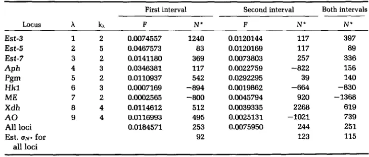
have also calculated estimates of N and of the standard errors of the estimates for the data of BEGON, KRIMBAS and LOUKAS (1980) on nine loci in a population of Drosophila subobscura on Mount Parnes. These figures are given in Table 2.

For these data the values given for tl and t 2 are 7 and 9 and So,

SI

and S2, respectively, equal to 190, 250 and 335 for all loci. The values of F and N for the first interval are obtained from the allele frequencies in Table 1 of BEGON, KRIMBAS, and LOUKAS (1980). Those for the second interval have been computed from their tabulated allele frequencies at times 7 and 9.

It may be seen from my Table 2 that there is considerable variability among the N" values that have been calculated for individual loci, and some of them are even negative. This is to be expected, even in the absence of selection,

TABLE 2

Estimates of N and of the standard errors of the estimates in the population observed by Begon, Krimbas and Loukas

First interval Second interval Both intervals

Locus kh F N * F N' N'

Est-3 Est-5 Est-7 APh Pgm Hkl ME Xdh A 0 All loci

Est. UN. for all loci

1 2 2 5 3 2 4 3 5 2 6 3 7 2 8 4 9 4

because (21) indicates that the sampling variance of N* between loci can be substantial in size. Our estimates of U N * for the other set of data are consistent

with this. However, the estimates from the data pooled over all nine loci are very much alike in the first and second intervals and are also of the same order of magnitude as the “temporal method” estimate given by BEGON, KRIMBAS and LOUKAS for the period between t = 0 and t = 7. In contrast, they are very much smaller than the temporal method estimate of N that they compute for period

2 as well as their estimates obtained by using “allelism of lethals” and the “ecological method.”

One possible cause of the discrepancies is, once again, local sampling of the flies, which would lead to underestimates if any variant of the temporal method, such as mine, is used. Another possibility is that the ratio of the variance of family size to the mean is underestimated by the figure of 14.38 used by BEGON,

KRIMBAS and LOUKAS (1980) in their application of the ecological method, because, as pointed out by HILL (1979), the variance that is relevant for popu- lations with overlapping generations is that of the number of offspring produced in a lifetime. This could be quite large in natural populations of insects that have very high mortality rates among young individuals. Moreover, it may be very difficult to estimate in such populations. If, in fact, the variance to mean ratio were greatly underestimated, this would result in a considerable overesti- mate of the effective population size.

I do not believe that, on the whole, this second set of data show much evidence for selection, although, as we shall see, selection would have to be strong for it to be detectable.

A COMPARISON OF VARIOUS METHODS

NEI and TAJIMA (1981) note that the maximum values of Fb and F, are 4 and

2, respectively, and also observe that it is possible for Fa to be infinite. It is then plausible to conjecture that F, should have a smaller variance than the other two statistics and their simulations lend support to this conjecture.

The statistic F K ~ should also be good, because, by (ll),

4 xilxio

8 1

=--

K

-

1 i=l x i ~

+

Xi0

Thus, its largest possible value is 4/(K - l), which is smaller than 2 if K

>

3. Let us therefore compare the variances of Fa, Fb, F, and F K ~ . First, we note that if dil

= xi1 - pi and dio = xi0 - p i are small,

where, as before, Vi1 = xi1 - xio. Hence, if there is no selection, (18) leads to the conclusion that

1 1 tl

E(Fc) z -

+

-

+

-,

EFFECTIVE POPULATION SIZE

which is the same as the approximate mean of Fm. In addition

543

Thus, if we apply expression (A8) and make use of the fact that V(vfl) = 2[E

vi^)]^,

we obtain

Therefore

This reasoning can also be applied to show that, if terms of the same order of magnitude as max (d?l, d & ) are neglected, the ri ht side of (30) is also approxi-

expression (A5) implies that

mately equal to V [ X T F a / E ( F a ) ] and V[

P-

K

-

lFb/E(Fb)]. In contrast to (30),

If K = 2, the right side of (30) is equal to 2. In this case F, is preferable to Fzl,

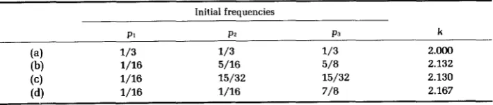
because F, has approximately the same mean and variance as FZI and a smaller maximum value. If, however, K = 3 , the maximum values of the two statistics are both equal to 2, so that their variances should be calculated to judge which statistic is to be preferred. I have done this for various sets of initial frequencies, using (30). The results are in Table 3.

The initial configurations are the same as those used by LEWONTIN and

KRAKAUER ( 1 9 7 3 ) in their Table 5 . The values of k = V[&FJE(F,)] that I have obtained are in approximate agreement with their simulations, there being consistency with respect to the ordering of the sizes of the k values for configurations (a), (b), (c) and (d). Our results indicate that F31 is preferable to

Fa, Fb and F, when K = 3 , particularly if the initial frequencies vary greatly.

TABLE 3

Approximate values of k = V[& Fc/E(Fc)] for various sets of initial frequencies

Initial freouencies

P 2 P 3 k

PI

1/3 1/3 1/3 2.000

(4

1/16 5/16 5/8

(b)

(4

(4

1/16 1/16 7/8

2.132

15/32 15/32 2.130

DISCUSSION

Most applications of the diffusion approximation in genetics, such as those described in detail by CROW and KIMURA (1970), can accommodate values of t

that are as large as integer multiples of N. Solutions can be obtained for small

t, but they are then series expansions that are complicated in form.

However, the situations discussed in this paper make it reasonable to assume that t/N is very small. This is because, in practice, a scientist would want to finish his project within a reasonable length of time, and there would be no need to estimate N indirectly by any of the methods discussed in this paper unless it is quite large. One is then led to a different sort of diffusion approxi- mation, which is not as good as the standard one when t/N is large, but may surpass it in leading to solutions that are simple and easily interpretable when this ratio is small.

This second approach has been used by VORONKA and KELLER (1975) in analyzing the behavior of populations with two alleles. I have adapted it to the multiple-allele situation and obtained expressions that generalize some of theirs. The calculations are in the APPENDIX.

The variances and covariances that are derived in the APPENDIX can also be computed directly for the Wright-Fisher model, after much tedious algebra. Thus, the mathematical treatment in the APPENDIX is preferable because of its relative simplicity. In addition, it has the merit of generality, because various authors have proved in the literature that the diffusion approximation is valid for a large class of discrete generation models, as well as the overlapping generation model of Moran. Examples of such work are the papers of WATTER-

SON (1962), FELDMAN (1966) and ETHIER and NAGYLAKI (1980). In addition, it has

already been mentioned that it is not necessary to have a constant N, because, if it varies with time, it can be replaced by

A,

the harmonic mean of the effective population sizes in the interval of time being considered.

Also, there have been, in recent years, several papers concerned with the derivation of N for age-structured populations. A general argument is given, for example, by HILL (1979). EMIGH (1979) has also shown that diffusion theory is applicable, at least to haploid age-structured populations, after a period, rela- tively short compared with the time scale of the process, in which the frequen- cies of a particular allele in various age groups approach a common value. Thus, if a population that is being studied has lived for a long time in its present habitat and is well adapted to it, the theory in this paper should be applicable. If this is not so, the shifts in allele frequencies may be larger than the theory predicts they should be. The size of FKr would then be increased. Furthermore, it should be noted that the treatment of EMIGH (1979) relies on the population having unchanging demographic parameters. The failure of this assumption to hold could also inflate the value of FKr and hence lead to an estimate of N that is too small in an age-structured population.

EFFECTIVE POPULATION SIZE 545

the effects of weak viability selection on the mean and variance of F e . The effects are indeed negligible. These results are consistent with those obtained by NICHOLAS and ROBERTSON (1975) in their study of the effects of selection on

Fa when there are two alleles. Their work implies that if t / N is small, the effects of additive or heterotic selection would not be detected, even with quite large selective differences between the genotypes.

It is also possible to relax another apparently restrictive assumption. For if

NA is much larger than N, it is not necessary to assume in the derivation of (15)

that N is equal to the number of reproducing individuals, which then have a binomial offspring distribution. We could have a more general effective popu- lation size. The assumption that NA >> N is very likely to be realistic for populations, such as those of insects, that have a high mortality rate among the young and high fertility among the survivors.

In summary, it seems likely that the temporal method for estimating N indirectly from F K ~ can give a reasonable rough estimate. If data can be collected on many alleles at several unlinked loci, the standard error may even not be extremely large in comparison with the point estimate. The method should be most effective for short-lived organisms with high mortality among the young and high fertility of the survivors, for then N

cc

NA, and any bias from the population not being in demographic equilibrium should be at a minimum.

The statistic F K I is simple in form because it is like a chi-squared statistic in which the unknown expected value in each denominator is replaced by a corresponding sample estimate. The figures in Table 3 also demonstrate that F ~ I

is less sensitive than

Fa,

Ft, and F, to variations in initial allele frequencies. If K

> 3, its advantage over the alternative statistics should be increased because the maximum value 4/(K

-

1) is less than 2. In addition, the theory in the APPENDIX indicates that it is

F K ~

that is approximately distributed as a multiple of a noncentral chi-squared random variable with K - 1 d.f., rather than Fa, F b , or

Fe.

Finally, another advantage of the approach discussed in this paper is that it provides a procedure for pooling information from two or more time intervals, as well as two or more unlinked loci. It seems that among previous authors, only NEI and TAJIMA (1981) have considered the latter and none have dealt with the former.

I am grateful to M. NEI for introducing me to this area of research. I also thank him, P. PAMILO and C. B. KRIMBAS for helpful suggestions. In addition, I am grateful to an anonymous reviewer for pointing out a serious error in an earlier version of this paper. This study was supported by National Institutes of Health grant GM-20293.

LITERATURE CITED

BEGON, M., C. B. KRIMBAS and M. LOUKAS, 1980 The genetics of Drosophila subobscuro popula- tions. XV. Effective size of a natural population estimated by three independent methods. Heredity 4 5 335-350.

CROW, J. F. and M. KIMURA, 1970 An Introduction to Population Genetics Theory. Harper & Row. New York.

EMIGH, T. H., 1979 The dynamics of finite haploid populations with overlapping generations.

ETHIER, S. N. and T. NAGYLAKI, 1980 Diffusion approximations of Markov chains with two time

FELDMAN, M. W., 1966 On the offspring number distribution in a genetic population. J. Appl. Prob.

HILL, W. G., 1979 A note on effective population size with overlapping generations. Genetics 92:

KRIMBAS, C. B. and S. TSAKAS, 1971 The genetics of Dacus oIeae. V. Changes of esterase polymor- phism in a natural population following insecticide control: selection or drift? Evolution 25 454-460.

11. The diffusion approximation. Genetics 92: 339-351.

scales and applications to population genetics. Adv. Appl. Probab. 12: 14-49.

3 129-141.

317-322.

LANCASTER, H. O., 1969 The Chi-Squared Distribution. John Wiley & Sons, Inc., New York. LEWONTIN, R. C. and J. KRAKAUER, 1973 Distribution of gene frequency as a test of the theory of

NEI, M. and F. TAJIMA, 1981 Genetic drift and estimation of effective population size. Genetics 98:

NICHOLAS, F. W. and A. ROBERTSON, 1976 The effect of selection on the standardized variance of

PAMILO, P. and S. L. VARVIO-AHO, 1980 Letter to the editor on the estimation of population size

SCHAPPER, H. E., D. YARDLEY and W. W. ANDERSON, 1977 Drift or selection: a statistical test of

SOURDIS, J. and C. B. KRIMBAS, 1980 On Pamilo and Varvio-Aho’s note about the estimation of

VORONKA, R. and J. B. KELLER, 1975 Asymptotic analysis of stochastic models in population

WATTERSON, G. A., 1962 Some theoretical aspects of diffusion theory in population genetics. Ann.

WILSON, S. R., 1980 Analyzing gene-frequency data when the effective size is finite. Genetics 95:

Corresponding editor: B. S. WEIR selective neutrality of polymorphisms. Genetics 7 4 175-195.

625-640.

gene frequency. Theor. Appl. Genet. 48: 263-268.

from allele frequency changes. Genetics 9 5 1055-1057.

gene frequency variation over generations. Genetics 87: 371-379.

effective population size. Genetics 96: 561-563.

genetics. Math. Biosci. 2 5 331-362.

Math. Stat. 33: 939-957.

489-502.

APPENDIX: SOME DISTRIBUTION THEORY

I shall assume that sampling scheme number 2 holds, because it is the one most likely to apply in practice. A similar theory can be developed for sampling scheme number 1. Notations that will be used are N(p, I:) for a normal random variable with mean p and covariance matrix I: and x h for a noncentral chi-squared random variable with r degrees of freedom and noncentrality parameter A. A symbol

-

between an algebraic expression and the symbol for a random variable shall denote that the expression is approximately distributed as the random variable.

Let Nt denote the variance effective population number at time t. Then, if t is much smaller than

N t , the frequency of the allele is unlikely to change much between times 0 and t . Hence, if there is, at most, weak viability selection and z, denotes the frequency of A, at time t and p, its frequency among adults at time 0,

EFFECTIVE POPULATION SIZE 547

where cu, is the effect of A,, on deviations of the relative viabilities 1

+

suu from 1 and-&, is Kronecker's delta. Thus, if we invoke a continuous approximation, the density function f(z, t ) of the allele frequencies at time t is a solution of the differential equation

where C,, = p,(S,, - p"). The solution of (AI) is

where pul = p.(l

+

h t ) , C is a constant such that f(z, t) integrates to 1 over the region

Thus, because allele frequencies pul are constrained to add to 1, (A2) implies that the vector z has a K - 1-dimensional normal distribution with mean vector pk = (pul) and covariance matrix [t(2fl)-']Z, where Z is a K X K matrix of rank K - 1. Therefore, because the samples at times 0 and

t are independent, and xo

-

N(p, (2So)-'X), where p = (pu), x

-

xo

-

N(p1 - p, [(2So)-'

+

t(2R)-']E). Hence

where

A=[&+-&] -l

z

(p.1

-

P d 2

-

[

-+-

2;o 2;]-1; u t

U-1 Pu and

d

= E,p,,a:.

Now let us consider time tl. Then (2N")-'t = (ZS1)-'

+

t1(2N)-'. Hence, it follows from the theory for the noncentral chi-squared random variable, as described, for example, by LANCASTER (1969), that (A3) and (11) lead to

1 1 tl t?uH

E(FKI) =a+-+-+-

2So 2S1 2N 2(K- 1) and

r

Results can be obtained for F K ~ by noting that it is equal to (K - I)-' X qK,j-l,jg where j-1

Since the same sort of sampling takes place between times tJ-] and t, as between times 0 and t1,

one can obtain analogues to (A4) and (A5) in which p,-1= (p+,) tJ

-

t,-1, ZS, and Z ~ , - I . respectively, replace p. tl, 2S1 and 2So, and the expectations are conditional upon P,-~. Since these expectations do not depend upon pJvl they are also equal to unconditional expectations. Consequently, we are led to

All that now remains in the derivation of V(FK,) is to obtain Cov(r+x,,-l.,, (PK.,,-I,,,), where j # m. First, if I j - m I 2 2 and t’ = min(t,-1, t,,-l), Cov(cpK,,-1.,. P)K,,,-I,,, I p t , ) = 0, because the samples at times t , and t] are independently drawn from the gene pool at time t ’ . Thus the unconditional covariance is also equal to zero. Second, if m = j - 1, we have, from (A3), that if wul, = xu,, - P..~, for j ’ = j , j - 1, j - 2, then

cov(’?K.l -1.1 9 CPK,, -2.1 -1 I PJ-2)

1 t,-, - t,-2

+

ZS,-i 2N K - 1

Therefore, it can be shown that

We conclude this appendix by sketching a derivation of the covariance of squares of allele frequency changes when there is no selection. It can be shown by using (A3) that vI1 and vC1

+

E V ~ ~ ,

where E is either 1 or -1, are respectively distributed as [(ZSo)-’

+

(ZSl)-’

+

t1(2N)-1]1’2N(0, p,(l - p,)) and [(2So)-’

+

(ZSl)-’ + t1(2N)-’]’’*N(O, p,(l - pz)

+

ph(1 - ph) - 2ep, ph). We may then obtain E(v:l) and use E[(vzl

+

vh1)4 - (vtl - Vhl)l] to obtain E[v?~vil]. Hence, we are led to

cov(v;l, V i l )

=

zp:pi - + - +

.