Available Online atwww.ijcsmc.com
International Journal of Computer Science and Mobile Computing
A Monthly Journal of Computer Science and Information Technology
ISSN 2320–088X
IMPACT FACTOR: 5.258IJCSMC, Vol. 5, Issue. 7, July 2016, pg.553 – 557
Interpolative Absolute Block Truncation
Coding for Image Compression
Dr. Ghadah Al-Khafaji
Baghdad University/Collage of Science/Computer Science Department/Iraq
Abstract: In this paper, an interpolation technique of nearest neighbour base is proposed along with absolute block truncation coding that exploited the spatial domain of low resolution image, and then reversely reconstruct the up layers hierarchically. The results showed the superior performance of compression ratio and image quality compared to traditional absolute block truncation coding.
Keywords: image compression, absolute block truncation coding and interpolation technique
1. Introduction
Compression techniques represent the cornerstone of all the multimedia areas, to efficiently compress large data files of huge bytes consumption of image, video, audio and audio.
Image compression techniques play a vital role in our live, resembling a heart for enabling technology [1], which simply based on utilizing the redundancy(s) of statistical base and/or human visual system (HVS) base, for the former one encompass the interpixel and coding redundancies, while for the latter one means the psychovisual redundancy, due to the redundancy type(s) exploited image compression classified into lossy and lossless. Reviews of image compression techniques can be found [2-7].
Block Truncation Coding (BTC) an effective lossy technique that characterized by simplicity, symmetry of encoder/decoder and efficient compression ratio due to the ability to represent the image information using the mean and standard deviation, thus sometimes referred to as moment-preserving block truncation because it preserves the first and second moments of each image block, but the main drawbacks of this technique are blocking effects and edge degradation [8].
2. The Proposed System
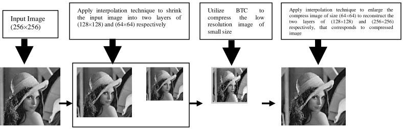
The implementation of the proposed system is explained in the following steps as shown in figure (1). The general idea behind the work of interpolation scheme base can be found in details in [9], which utilized the traditional prediction coding techniques.
Step 1: Load the input uncompressed gray image Y0 of BMP format of size N×N that corresponds to high
resolution image of size 256×256 that resemble to layer0 or root of the tree.
Step 2: Apply the interpolation technique of multiresolution scheme through shrinking and enlarging base. Different interpolation techniques can be utilized ranging from the simple and easy, like the nearest neighbour approach, to more accurate ones like the bi-linear technique adopted in this work, to complex ones like higher order interpolation. The choice between them depends on the speed, computations and quality desired [1]. In this paper the simple popular nearest neighbour interpolation techniques used, where the interpolation technique works by creating the medium resolution image Y1 and low resolution image Y2
each of size (N/2×N/2) and (N/4×N/4) respectively corresponds to layer1 and layer2, namely create the
smaller Y1 of size 128×128 from the original Y0 and then create Y2 of size 64×64 from the shrinked Y1 [10].
Step 3: Perform the absolute block truncation coding (ABTC) on the low resolution image Y2 (layer2) of
two levels (1 bit) quantizer of moment base, using the following sub steps [11]:
1. Computer first moment value, namely mean, for each block of size (n×n), then the image block values grouped into two ranges of values, namely upper range is those gray levels which are greater than the block average gray level (x) and the remaining brought into the lower range. The mean of higher range XH and
the lower range XLare calculated as: n i i Y n x 12 ) 1 ( 1
Where Y2i represents the ith pixel value of the low resolution image block (layer2 image block) and n is the
total number of pixels in that block.
(3) ) ( 1 (2) 1
2
n x xi i L n x xi i H x K n X x K X
Here K is the number of pixels whose gray level is greater than x, and n2 is the block size.
2. Create the Binary image block, denoted by B (two-level bit plane image) that is obtained by comparing each value Y2i with the threshold value (i.e., block mean), in other words’1’used to represent a pixel whose
gray level is grater than or equal to mean (x) and ‘0’ to represent a pixel whose gray level is less than mean (x).
) 4 ( x i Y if 0 x i Y if 1 2 2 B
3. Apply entropy encoder of the compressed information of low resolution image (ABTC binary image and coefficients) using run length coding of binary image and LZW to XH and XL respectively.
4. Reconstruct the compressed approximated image of low resolution base, an image block Y~2 is reconstructed by replacing the `1’ s with XH and the ’0’'s by XL.
(5) 1 0 ~ H L 2 B X B X Y
Step 4: Use lower resolution image information (layer2) to reconstruct the medium layer (layer1), such as:
1. Apply the nearest neighbour interpolation concept to create the enlarged image InMed[Y~2] of medium size resolution 128×128 from the approximated image Y~2 of size 64×64.
2. Find the first residual image as a difference between the original shrinked image of medium resolution Y1
and the interpolated one from the step above.
) 6 ( ] ~ [2 1
1 Y In Y
e Med
) 7 ( )
( 1 1 1 1
1 1 e e QS Q e D e QS e round Q
e
4. Find the approximated medium resolution image Y~1as a sum of interpolated one InMed[Y~2] along with the dequantized residual, such as:
) 8 ( ] ~ [ ~ 1 2
1 In Y eD
Y Med
Step 5: Build the high image resolution (layer0 or root) of same size as the original using the medium
constructed layer above (layer1), such as:
1. Use the nearest neighbour interpolation concept to create the enlarged image InHgt [Y~1] of high size resolution 256×256 from the approximated image Y~1 of size 128×128 (see, Step 4 above).
2. Find the second residual image as a difference between the original image of high resolution Y0 and the
interpolated one resultant from the step above.
) 9 ( ] ~ [1 0
0 Y In Y
e Hgt
3. Quantize/dequantized the second residual image using the simple uniform scalar quantizer, such as:
) 10 ( )
( 0 0 0 0
0
0
e
e e D e Q QS
QS e round Q
e
4. Find the approximated high resolution image Y~0as a sum of interpolated one InHgt[Y~1] along with the dequantized residual image, such as:
) 11 ( ] ~ [ ~ 0 1
0 In Y e D
Y Hgt
In addition to low resolution image information (ABTC binary image & coefficients), the dequantized differences of medium and high resolutions layer respectively, encoded using the LZW techniques.
3. Experimental & Results
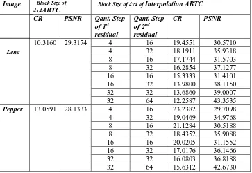
In order to evaluate the performance of the proposed compression technique compared to the ABTC method that applied to standard images as shown in figure 2 also the 4×4 block size used along with various quantization level/steps of first and second residual images.
Table (1) illustrated the results in terms of objective fidelity criteria of Peak Signal to Noise Ratio (PSNR) (see equation 12) between the original image Y0and the decoded (compressed) image Y~0, and the Compression Ratio (CR) (see equation13).
(~( , ) ( , )
(12)1 255 log . 10 1 0 1 0 2 0 0 2 10 N x N y y x Y y x Y N N PSNR
Fig. (1): The proposed compression system structure.
Input Image (256×256)
Apply interpolation technique to shrink the input image into two layers of (128×128) and (64×64) respectively
Utilize BTC to compress the low resolution image of small size
) 13 ( Im
rmation ressedInfo SizeofComp
age inal SizeofOrig nRatio
Compressio
The results showed elegant performance, where the compression ratio improved compared to the traditional
ABTC with higher image quality. This is due to utilization the interpolation technique that leads to the construction of low resolution image of small error quality that reconstructed hierarchically.
Certainly, the quality of the decoded image is improves as the number of quantization levels of both of the residual images of two layers (layer2 and layer1). The main disadvantage of increasing the quantization
levels, however, lies in increasing the size of the compressed information. It is a trade-off between the desired quality and the consumption of bytes; the higher the quality required, the larger the number of quantization levels that must be used. While the traditional ABTC affected by the mean value corresponds to threshold value (i.e., mean) .
Lastly, this technique work by exploiting the spatial domain base, which implicitly means, the results varies according to image details, where for simple image details higher performance achieved than higher or complex image details.
Table 1: Comparison performance between traditional ABTC and Interpolative ABTC techniques for tested images, where all the images are square gray scale images of size 256x256 pixels of 8 bit/per pixel.
Image Block Size of 4x4ABTC
Block Size of 4x4 of Interpolation ABTC
CR PSNR Qant. Step
of 1st residual
Qant. Step of 2nd residual
CR PSNR
10.3160 29.3174 4 16 19.4551 30.5710
4 32 18.1911 35.9318
8 16 17.1744 31.5703
8 32 16.2854 37.1277
16 16 15.3333 31.4101
16 32 13.9800 38.1150
32 32 13.6860 39.0007
32 64 12.2587 43.3535
Pepper 13.0591 28.1333 4 16 23.2382 29.7098
4 32 19.0469 34.9768
8 16 21.1284 30.5188
8 32 18.4352 35.9088
16 16 20.0205 31.1552
16 32 17.0176 36.1466
32 32 16.0803 36.8188
32 64 15.6312 42.6730
Lena
a b
e a
4. Conclusions
It is obvious that the proposed technique of interpolation base or multiresolution layers, that reversely uses the hierarchical down layers to reconstruct the up layers, improves the performance compared to traditional
ABTC, even here the simple popular interpolation technique of nearest neighbour used.
References
1. Al-Khafaji, G. 2012. Intra and Inter Frame Compression for Video Streaming. Ph.D. thesis, Exeter University, UK.
2. Gonzalez, R. C. and Woods, R. E. 2003. Digital Image Processing 2nd edn. Prentice Hall.
3. Sayood, K. Introduction to Data Compression. 2006. 3rd edn.Elsevier Inc., San Francisco United States of America.
4. Vijayvargiya, G., Silakar,i S. and Pandey R. 2.13. A Survey: Various Techniques of Image Compression, International Journal of Computer Science and Information Security, 11(10),51-55.
5. Khobragede, P. and Thakare, S. 2014. Image Compression Techniques-A Review International Journal of Computer Science and Information Technologies, 5(1),272-275.
6 Rasha, Al-T. 2015. Image Compression Using Enhancement Polynomial Prediction Coding .MSc. thesis, Baghdad University, Collage of Science.
7. Mahdi N.S. 2015. Image Compression based on Adaptive Polynomial Coding. Diploma, Dissertation, Baghdad University, Collage of Science.
8. Al-Khafaji, G.2013. Hybrid Image Compression based on Polynomial and Block Truncation Coding. Electrical, Communication, Computer, Power, and Control Engineering (ICECCPCE), 2013, International Conference on Mosul, IEEE.
9. Burgett, S. and Das, M. 1993. Predictive Image Coding using Multiresolution Multiplicative Autoregressive Models. Proceedings of the IEEE, 140(2), 127-134.
10. Athraa, T. 2015. Adaptive Polynomial Image Compression. Diploma, Dissertation, Baghdad University, Collage of Science.