LP Solutions of Vectorial Integer Subset Sums –
Cryptanalysis of Galbraith’s Binary Matrix LWE
Gottfried Herold and Alexander May
Horst G¨ortz Institute for IT-Security Ruhr-University Bochum, Germany
Faculty of Mathematics
[email protected],[email protected]
Abstract. We consider Galbraith’s space efficient LWE variant, where the (m×n)-matrixA is binary. In this binary case, solving a vectorial subset sum problem over the integers allows for decryption. We show how to solve this problem using (Integer) Linear Programming. Our attack requires only a fraction of a second for all instances in a regime formthat cannot be attacked by current lattice algorithms. E.g. we are able to solve 100 instances of Galbraith’s small LWE challenge (n, m) = (256,400) all in a fraction of a second. We also show under a mild assumption that instances withm ≤2n can be broken in polynomial time via LP relaxation. Moreover, we develop a method that identifies weak instances for Galbraith’s large LWE challenge (n, m) = (256,640).
Keywords:Binary matrix LWE, Linear Programming, Cryptanalysis
1
Introduction
Over the last decade, the Learning with Errors (LWE) problem [17] has proved to be extremely versatile for the construction of various cryptographic primitives. Since LWE is as hard as worst-case lattice problems, it is consider one of the most important post-quantum candidates. Let us recall that an LWE instance consists of a random (m×n)-matrix A with elements from Zq and an m-dimensional
vectorb∈Zm
q , whereb=As+emodqwith a secret randoms∈Znq and where
the entries ofe∈Zm
q are from a discretized normal distribution.
The LWE decisional problem is to distinguish (A,b) from (A,u) for random
u∈Zm
q . While LWE has some intriguing hardness properties, it is known that
one has to choose quite largenin order to reach a desired security level against lattice reduction attacks. This in turn makes the size of LWE instances (A,b), and thus the size of public keys, undesirably large. For practical reasons, people therefore looked into various variants of LWE, such as ring-LWE [14,15], LWE
with short secret [16,2] or LWE with short error [16,10]. Recently, some special instances of ring-LWE were identified to have serious weaknesses [6,4], but these instances were not suggested for cryptographic use. Moreover, it was shown that LWE with binary secrets and errors can be attacked in slightly subexponential time 2O(n/log logn)by a BKW-type algorithm[12], where LWE dimensionn= 128
was practically broken within half a day. Also, LWE with binary secret leads to more efficient lattice attacks [3]. While choosing special variants of LWE seems to slightly decrease the security, the improved attacks do not substantially endanger the security of these variants in general.
In this paper, we look at another LWE variant due to Galbraith [8]. In this variant,A is replaced by abinary matrix. This makes Galbraith’s variant very tempting for low-weight devices that are not capable of storing a sufficiently large LWE instance.
In [8], Galbraith instantiates Regev’s encryption system [17] with his binary matrix A and suggests to use the parameters (n, m, q) = (256,640,4093) that were originally proposed by Lindner and Peikert [13] for Regev’s original scheme. Galbraith also gives a thorough security analysis based on lattices, where in his experiments he fixesnand tries to break encryption for increasingm. Based on this analysis, he concludes that instances withm≥400 might be hard to break with lattice techniques.
For Regev’s original scheme, security follows from hardness of LWE for ap-propriate parameters; this is not automatically the case for binary matrix A
without changing parameters. For Galbraith’s choices, in order to break en-cryption, one can solve an equation of the form uA= c1 for a known matrix A∈ {0,1}m×n, some known ciphertext component c
1∈Zn and some unknown vector u ∈ {0,1}m. In other words, one has to find a subset of all rows of A
that sums to c1. We call this problem therefore a vectorial integer subset sum.
If the unknown vector u is short, a vectorial integer subset sum can certainly be solved by finding a closest vector in some appropriate lattice. This is the standard analysis that was carried out in [8] against this avenue of attack.
However, a vectorial integer subset sum is by its definition also an Integer Linear Programming (ILP) problem. Namely, we are looking for an integral solution u ∈ Zm of m linear equations over the integers. While it is known that ILP is in general NP-hard, it is also known that in many cases removing the integrality constraint on u provides a lot of useful information about the problem. Removing the integrality constraint is called a LP relaxation of the problem. Without integrality constraints, the resulting problem can be solved in polynomial time, using e.g. the ellipsoid method [9].
regime formthat seems to be infeasible to reach with current lattice reduction algorithms.
However, m ≤ 2n does not quite suffice to break Galbraith’s (n, m) = (256,640)-challenge in practice. Namely, when we look at instances withm >2n the success probability of our MATLAB ILP solver drops quite quickly – when we allow only some fixed, small computation time. Yet, when looking at a large number of instances of our vectorial integer subset sums, we realize experimen-tally that there is still a significant number of weak instances that are vulnera-ble to LP relaxation with some additional tricks (such as e.g. the cutting plane method). More concretely, we are able to show that at least 1 out of 215instances
of Regev-type encryptions with (n, m) = (256,640) can be solved in about 30 minutes. Interestingly, we are able to compute a simple score for every instance Ithat accurately predicts whetherIis indeed weak – based on an estimation of the volume of the search space that comes from the LP relaxation. We find that such a quick test for identifying weak instances I is a quite remarkable prop-erty of Linear Programming. We are not aware of a similar propprop-erty for other cryptanalytic methods. We hope that our results motivate more cryptanalytic research using (Integer) Linear Programming.
Note that our attack breaks Galbraith’s instantiation of LWE encryption with binary matrices, but does not break binary LWE itself. Due to that, our attack allows ciphertext recovery, but not key recovery.
Our paper is organized as follows. In Section 2, we recall Galbraith’s scheme and its cryptanalysis challenges. In Section 3, we model vectorial integer subset sums in form of an Integer Linear Programming. We attack instances withm≤
2nin Section 4 and show that they actually admit a polynomial time attack. In Section 5, we show how to identify weak instances for large mand we present our experimental results for Galbraith’s large challenge (n, m) = (256,640).
2
Galbraith’s Binary Matrix LWE
Let us briefly recall Regev’s LWE encryption scheme. Letqbe prime. One chooses a public A ∈R Zmq×n and a private s ∈R Znq. One then compute b = As+
emodq, where the ei are sampled from a discrete normal distribution with
mean 0 and standard deviationσ. The public key consists of (A,b).
For encrypting some messageM ∈ {0,1}, one chooses a random nonceu∈R
{0,1}mand computes the ciphertext
c= (c1, c2) = (uAmodq,hu,bi+M q
2
modq)∈Znq ×Zq.
For decryption to 0 respectively 1, one checks whether c1s−c2 is closer to 0
respectively q2.
After analyzing lattice attacks, Lindner and Peikert [13] suggest to use the parameters
for medium security level and estimate that these parameters offer roughly 128-bit security. However, for these parameters the public key (A,b) has already 247 kilobytes, which is way too much for constrained devices.
Therefore, Galbraith [8] suggested to construct the public matrix A with
binary entriessimply from the seed of a PRNG. All that one has to store in this case is the seed itself, and the vectorb. A similar trick is also used in other contexts to shorten the public key size [5].
Moreover, Galbraith gives a thorough security analysis of his LWE variant, based on its lattice complexity. In his security analysis he considers the problem of recovering the nonceufrom
c1=uA. (1)
Notice that since nowA∈ {0,1}m×n, every entry ofc
1is an inner product of two
random binary length-m vectors. Thus, the entries of c1 are random variables
from a binomial distributionB(m,14) with expected value m4. Since m4 q, the equalityc1=uAdoes not only hold moduloq, but also over the integers.
Hence, recoveringufrom (c1,A) can be seen as avectorial integer subset sum
problem. Once u is recovered, one can easily subtract hu,bi from c2 and thus
recover the messagem. Hence, solving the vectorial integer subset sum problem gives aciphertext only message recovery attack.
We would like to stress that this attack does not allow for key recovery ofs. We also note that in Regev’s original scheme, the security proof shows IND-CPA security assuming that the LWE problem is hard. For this reduction, we need thatc1is essentially independent ofA, which is proven using the Leftover Hash
Lemma by setting parameters sufficiently large. In particular, u is required to have sufficient entropy and Eq. (1) has many solutions for u in Regev’s non-binary scheme, whereas the parameters in Galbraith’s non-binary scheme are set such that uis the unique solution to Eq. (1). Due to that, our attack does not give an attack on binary LWE. In fact, binary LWE was shown to be at least as secure as standard LWE in [1], providedn is increased by a factorO(logq). Consequently, it seems unlikely that the attack extends to binary LWE.
2.1 Previous Cryptanalysis and Resulting Parameter Suggestions
In his security analysis, Galbraith attacks the vectorial integer subset sum by lattice methods. Namely, he first finds an arbitrary integer solution w ∈ Zm
withc1=wA. Then he solves CVP with target vectorw in the lattice
L={v∈Zm|vA≡0 modq}.
Letv be a CVP-solution, then we usually haveu=w−v.
Based on his analysis, Galbraith raised the two following cryptanalysis chal-lenges:
– C1 with (n, m) = (256,400): The goal is to computeu from (A, c1) in less
than a day on an ordinary PC.
– C2 with (n, m) = (256,640): The goal is mount an attack using current computing facilities that would take less than a year.
According to Galbraith, breaking C1 should be interpreted “as causing em-barrassment to the author”, while C2 should be considered a “total break”.
3
Modeling our Vectorial Integer Subset Sum as an
Integer Linear Program
In the canonical form of an Integer Linear Program (ILP), one is given linear constraints
A0x≤b0,x≥0 andx∈Zm,
for which one has to maximize alinear objective functionhf,xifor somef ∈Rm that can be freely chosen.
Notice that it is straightforward to map our vectorial integer subset sum problemuA=c1 from Eq. (1) into an ILP. Namely, we define the inequalities
ATu≤c1
−ATu≤ −c 1and
ui≤1 for all i= 1, . . . , m.
ui≥0 for all i= 1, . . . , m.
(2)
We can for simplicity chosef = 0, since we are interested in any feasible solution to Eq. (2), and it is not hard to see that by the choice of our parameters our solutionuis a unique feasible solution. Namely, look at the map
{0,1}m→B m,1 4
n
,
u7→uA,
where X ∼ B(m,1
4) is a binomially distribution random variable with m
ex-periments and Pr[X = 1] = 1
4 for each experiment. Notice that the j
th entry,
1 ≤j ≤n, of uAcan be written as u1a1,j +. . .+umam,j, where we have the
event Xi thatuiai,j= 1 iffui=ai,j= 1, i.e. with probability 14. Hence, we can
model the entries ofuAas random variables from B(m,14).
For the usual parameter choice q > m, the solution u of Eq. (2) is unique as long as this map is injective, i.e. as long as the entropy of B(m,14)n
is larger thanm. The entropy of the binomial distribution B(m,1
4) n
is roughly
n
2log2( 3
4
Attacking
m
≤
2n: Solving Challenge C1
We ran 100 instances of Eq. (2) on an ordinary 2.8 GHz laptop withn= 256 and increasingm. We used the ILP solver from MATLAB 2015, which was stopped whenever it did not find a solution after time tmax = 10 seconds. We found
that the success probability of our attack dropped from 100% at m = 490 to approximately 1% atm= 590, cf. Table 1. The largest drop of success probability takes place slightly afterm= 2n.
For comparison, we also solved the LP relaxation, i.e. Eq. (2) without inte-grality constraint onu. This is much faster than ILP, so we solved 1000 instances for eachm. We checked whether the returned non-integral solution matched our desired integral solution foru, in which case we call a run successful. The success rate of LP relaxation is also given in Table 1.
It turns out that Galbraith’s small C1 challenge can already solely be solved by its LP relaxation. Since LP relaxation is only the starting point for ILP, it does not come as a surprise that ILP has a slightly larger success rate. However, it is impressive that LP relaxation alone is already powerful enough to solve a significant fraction of all instances.
m 400 450 480 490 500 510 512 520
Success(ILP) 100% 100% 100% 100% 96% 83% 79% 63%
Success(LP) 100% 99.6% 93.3% 82.3% 68.8% 55.6% 48.1% 35.4%
m 530 540 550 560 570 580 590 600
Success(ILP) 60% 32% 25% 12% 3% 1% 1% 0%
Success(LP) 19.8% 11.0% 4.5% 1.9% 0.8% 0.3% 0% 0%
Table 1.Success probability for solving Eq. (2) forn= 256. We used MATLAB 2015 and restricted totmax= 10 seconds for the ILP.
We now give a theoretical justification for the strength of LP relaxation, showing that under some mild heuristic, for m ≤ 2n, the solution of the LP relaxation is unique. Since, by construction, we know that there is an integral solution u to Eq. (2), uniqueness of the solution directly implies that the LP solver has to find the desiredu.
In the following lemma, we replace our linear constraints from A by some random linear constraints from some matrix ¯A over the reals. This will give us already uniqueness of the solution u. Afterwards, we will argue why replacing
¯
Aback by our LWE matrixAshould not affect the lemma’s statement.
Lemma 1. Let u∈ {0,1}2n. LetA¯ ∈
Rn×2n be a random matrix, whose rows
are uniformly distributed on the sphere around0∈R2n. Then
Proof. Let us look at the 2n-dimensional unit cubeU2n ={x∈(R∩[0,1])2n}. Obviously 0,u∈ U2n, both lying at corners of U2n. Now, let us assume wlog.
that u = 0 (which can be achieved by reflections). Let H be the hyperplane defined by the kernel of ¯A.
Since ¯Ais randomly chosen fromRn×2n, it has full ranknwith probability 1:
since we chose the entries of ¯A from the reals R, we avoid any problems that might arise from co-linearity. Thus,H as well as its orthogonal complementH⊥ have dimension n. Notice that H⊥ = Im( ¯AT). By construction, both H and
H⊥ intersect U2n in the corner 0 = u. We are interested whether one of the
hyperplanes goes throughU2n.
The answer to this question is given by Farkas’ Lemma [7], which tells us
thatexactly oneofH andH⊥passes throughU2n. Notice first that not both can
pass through U2n. Now assume that H intersectsU2n only in the zero point0.
Then Farkas’ Lemma tells us that there is a vector in its orthogonal complement H⊥that fully intersectsU2n. Notice that again by having vectors over the reals,
the intersectionH⊥∩U2n isn-dimensional.
By the randomness of ¯A, the orientation ofH in R2n is uniformly random, and hence the same holds for the orientation of H⊥. Since H and H⊥ share exactly the same distribution, and since by Farkas’ Lemma exactly one out of both has a trivial intersection withU2n, we have
Pr[H∩U2n={u}] = Pr[H⊥∩U2n={u}] =
1 2.
Letb= ¯Au=0. SinceH = ker( ¯A), it follows thatuis a unique solution to the equation ¯Ax=bin the case thatH has trivial intersection with U2n. ut
Theorem 1. Under the heuristic assumption that our matrix AT behaves like
a random (n×m)-matrix, whose rows are uniformly distributed on the sphere
around0m, LP relaxation solves Eq.(2) in polynomial time for allm≤2n.
Proof. Notice that the case m = 2n follows directly from Lemma 1, since LP
relaxation has to find the unique solutionu, and its running time is polynomial using e.g. the ellipsoid method. For the case m < 2n we can simply append 2n−madditional columns toAT, and add a random subset of these toc
1.
Now let us say a word about the heuristic assumption from Theorem 1. Our assumption requires that the discretized AT defines a random orientation of a
hyperplane just as ¯A. SinceAThas by definition only positive entries, its columns
always have non-negative inner product with the all-one vector 1n. This minor
technical problem can be fixed easily by centering the entries ofATaround 0 via
the following transformation of Eq. (2):
First, guess the Hamming weight w = Pm
i=1ui. Then subtract (12, . . . , 1 2)
from every column vector ofAT and finally subtract w
2 from every entry ofc1.
After this transformation AT has entries uniform from {±1
2} and should fulfill
5
Attacking
m
= 640: Solving Challenge C2
In order to tackle them= 640 challenge, we could in principle proceed as in the previous section, identify a weak instance for e.g.m= 590, brute-force guess 50 coordinates of uand run each time an ILP solver for 10 seconds.
However, we found out experimentally that even in dimensionm= 640 the density of weak instances is not negligible. Hence, it seems to be much more effective to identify weak instances than to brute-force coordinates. So in the following we try to identify what makes particular instances weak.
We follow the paradigm that an ILP is the easier to solve, the more the LP relaxation “knows about the problem”. In particular, we expect that a problem is easy to solve if the solution polytope P of the LP relaxation of Eq. (2) is small. In the extreme case, if P ={u}, then the problem can be solved by the LP solver alone (cf. Thm. 1). To quantify the size of the solution space in an easy-to-compute way, we compute the length of a random projection of P. It turns out that this length, henceforth calledscore gives a very good prediction on the hardness of an instance.
More concretely, for an instanceI= (A,c), we choose a vectorrwith random direction. Then we maximize and minimize the linear objective function hr,ui
under the linear constraints given by the LP relaxation of Eq. (2) and consider their differenceD. Clearly,Sr := kDrkis the length of the orthogonal projection of
P onto the span ofr. Formally, thescore of an instanceIwrt. to some direction
r is defined as follows.
Definition 1. Let I = (A,c)be an instance. Consider the solution polytope P
of the LP relaxation of Eq.(2), i.e.P is defined asP = [0,1]m∩ {x|ATx=c}.
Let r∈Rm. Then the scoreSr is defined via
fmax:= max x∈Phr,xi
fmin:= min x∈Phr,xi
Sr :=
fmax−fmin krk
(3)
Note that Sr can be computed by solving two LP problems, hence in polynomial
time.
SinceSr quantifies the search space for the ILP, instances with small score
should be easier to compute. For m = 640, we computed the scores of 219
instances, which took approximately 1 second per instance.
Independence of r and Reliability of Our Score.We experimentally con-firm that for a given instance I, the value of Sr is mainly a function ofI and
does not depend significantly on the particular choice ofr. Therefore, we choose the fixed vector r = (1, . . . ,1,−1, . . . ,−1) for r with exactly m2 ones and m2
−1’s. We use the scoreS=Sr for this particular choice ofr and sort instances
We confirm that the scoreS is a very good predictor for the success of ILP solvers and the success probability drops considerably at some cutoff value forS. E.g. form= 520 and within a 10 second time limit, we find that we can solve
• >99% of instances withS≤1.22,
• 60% of instances with 1.22≤S≤1.54 and
• <3% of instances withS >1.54.
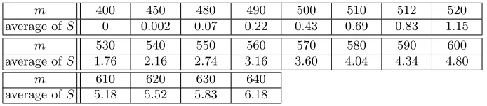
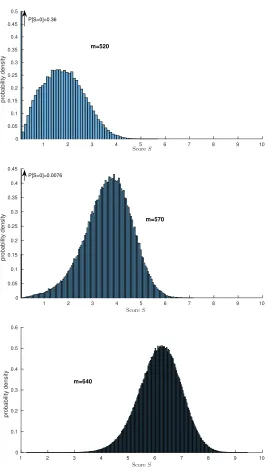
Distribution of S.Average values forScan be found in Table 2. Fig. 1 shows the distribution ofS. Note that while the distribution looks suspiciously Gaus-sian for m= 640, there is a considerable negative skewness and the tail distri-bution towards 0 is much fatter than for a Gaussian (cf. Fig. 2). This fat tail enables us to find a significant fraction of weak instances even for large m.
Notice that a score S = 0 basically means that LP relaxation finds the solution.
m 400 450 480 490 500 510 512 520
average ofS 0 0.002 0.07 0.22 0.43 0.69 0.83 1.15
m 530 540 550 560 570 580 590 600
average ofS 1.76 2.16 2.74 3.16 3.60 4.04 4.34 4.80
m 610 620 630 640
average ofS 5.18 5.52 5.83 6.18
Table 2. Average values for S for n = 256 and varying m. We used 1000 instances for eachm.
Results for m= 640.We generated a large numberN = 219 of instances with n= 256, m= 640, and tried to solve only those 271 instances with the lowest score S, which in our case meant S < 3.2. We were able to solve 16 out of those 271 weakest instances in half an hour each. We found 15 instances with S < 2.175, of which we solved 12. The largest value of S, for which we could solve an instance, was S≈2.6.
Fixing Coordinates. Let us provide some more detailed explanation why an ILP solver works well on instances with small score S. Consider some r ∈ {0,±1}m of low Hamming weight |r|
1 = w, so krk = √
w. Heuristically, we expect that Sr should be approximately S, as Sr mainly depends on the
in-stance and not on the choice ofr. Of course, for a vectorr∈ {0,±1}mwith low
Hamming weight we have
Sr =
1
√
w
max
x∈Phr,xi−minx∈Phr,xi
≤ √1
w
max
x∈[0,1]mhr,xi−x∈min[0,1]mhr,xi
=√w,
but that only means we should expect Sr to be even smaller. Since we know
ScoreS
1 2 3 4 5 6 7 8 9 10
probability density
0 0.05 0.1 0.15 0.2 0.25 0.3 0.35 0.4 0.45 0.5
m=520 P[S=0]=0.36
ScoreS
1 2 3 4 5 6 7 8 9 10
probability density
0 0.05 0.1 0.15 0.2 0.25 0.3 0.35 0.4 0.45
m=570 P[S=0]=0.0076
ScoreS
1 2 3 4 5 6 7 8 9 10
probability density
0 0.1 0.2 0.3 0.4 0.5 0.6
m=640
ScoreS
1 2 3 4 5 6 7 8 9 10
Number of instances
0 500 1000 1500 2000 2500 3000 3500
Normal Fit to Distribution of S for n=256, m=640
Total Number of Instances: N=524288
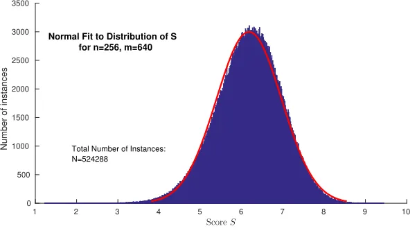
Fig. 2. Comparison of distribution of S for n = 256, m = 640 with a normal distribution. The distribution ofS has negative skewness and a much fatter tail towards 0. Hence, we obtain more weak instances than we would expect from a normal distribution.
hr,ui ≤ bfmaxcand hr,ui ≥ dfmineto the set of equations, where fmax resp.
fmin are the maximum resp. minimum computed forSr.
This is a special case of what is calledcut generationin Integer Linear Pro-gramming. IfSr <
√
w, i.e.fmax−fmin< w, then adding such a new inequality
always makes the solution space of the LP relaxation smaller. In fact, such an inequality restricts the possible set thatwout of the mvariablesui can jointly
obtain. So if Sr < √
w for many different r, we get lots of sparse relations between the ui. Such inequalities are calledgood cuts.
In particular, consider the casew= 1 andr= (0,0, . . . ,0,1,0, . . . ,0), i.e. we maximize / minimize an individual variableui overP. If this maximum is<1,
we know that ui = 0 holds and if the minimum is >0, we knowui = 1. So if
Sr <1 holds for somerwith|r|1= 1, we can fix one of theui’s and reduce the
number of unknowns by one – which makes fixing furtherui’s even easier. If the
scoreS is small, we expect that the ILP solver can find lots of such good cuts, possibly even cuts withw= 1.
Indeed, in all instances that we could solve, some variables could be fixed by such good cuts withw= 1. For dimensionsm≤550, most instances that were solved by the ILP could be solved by such cuts alone.
6
Conclusion
According to Galbraith’s metric for the challenge C2 in Section 3, the results of Section 5 can be seen as total break for binary matrix LWE. On the other hand, one could easily avoid weak instancesIby simply rejecting weakI’s dur-ing ciphertext generation. This would however violate the idea of lightweight encryption with binary matrix LWE.
Still, during our experiments we got the feeling that the vectorial integer subset sum problem gets indeed hard for largem, even for its weakest instances. So Galbraith’s variant might be safely instantiated for largem, but currently we find it hard to determinem’s that fulfill a concrete security level of e.g. 128 bit. One possibility to render our attack inapplicable is to change parameters such that modular reductions modqoccur in Eq. (1), since our attack crucially relies on the fact that we work overZ. Note here that while there are standard ways to model modular reduction via ILP asc1=uA−kq, this renders LP relaxation
useless: by allowing non-integralk, we can choose any value forc1,u.
Acknowledgements: The authors would like to thank Bernhard Esslinger and Patricia Wienen for comments.
Gottfried Herold was funded by the ERC grant 307952 (acronym FSC).
References
1. D. Boneh, K. Lewi, H. W. Montgomery, and A. Raghunathan. Key homomor-phic PRFs and their applications. In R. Canetti and J. A. Garay, editors,
CRYPTO 2013, Part I, volume 8042 of LNCS, pages 410–428, Santa Barbara, CA, USA, Aug. 18–22, 2013. Springer, Heidelberg, Germany. 4
2. Z. Brakerski, A. Langlois, C. Peikert, O. Regev, and D. Stehl´e. Classical hardness of learning with errors. In D. Boneh, T. Roughgarden, and J. Feigenbaum, editors,
45th ACM STOC, pages 575–584, Palo Alto, CA, USA, June 1–4, 2013. ACM Press. 2
3. J. A. Buchmann, F. G¨opfert, R. Player, and T. Wunderer. On the hardness of LWE with binary error: Revisiting the hybrid lattice-reduction and meet-in-the-middle attack. IACR Cryptology ePrint Archive, 2016:89, 2016. 2
4. W. Castryck, I. Iliashenko, and F. Vercauteren. Provably weak instances of ring-lwe revisited. Eurocrypt 16, 2016. 2
5. J.-S. Coron, D. Naccache, and M. Tibouchi. Public key compression and modulus switching for fully homomorphic encryption over the integers. In D. Pointcheval and T. Johansson, editors,EUROCRYPT 2012, volume 7237 ofLNCS, pages 446– 464, Cambridge, UK, Apr. 15–19, 2012. Springer, Heidelberg, Germany. 4 6. Y. Elias, K. E. Lauter, E. Ozman, and K. E. Stange. Provably weak instances of
ring-LWE. In R. Gennaro and M. J. B. Robshaw, editors,CRYPTO 2015, Part I, volume 9215 of LNCS, pages 63–92, Santa Barbara, CA, USA, Aug. 16–20, 2015. Springer, Heidelberg, Germany. 2
8. S. D. Galbraith. Space-efficient variants of cryptosystems based on learning with errors. https://www.math.auckland.ac.nz/ sgal018/pubs.html, 2013. 2, 4
9. M. Gr¨otschel, L. Lov´asz, and A. Schrijver.Geometric algorithms and combinatorial optimization, volume 2. Springer Science & Business Media, 2012. 2
10. T. G¨uneysu, V. Lyubashevsky, and T. P¨oppelmann. Practical lattice-based cryp-tography: A signature scheme for embedded systems. In E. Prouff and P. Schau-mont, editors,CHES 2012, volume 7428 ofLNCS, pages 530–547, Leuven, Belgium, Sept. 9–12, 2012. Springer, Heidelberg, Germany. 2
11. G. Herold and A. May. LP solutions of vectorial integer subset sums — crypt-analysis of Galbraith’s binary matrix LWE. In S. Fehr, editor,PKC 2017, Part I, volume 10174 of LNCS, pages 3–15, Amsterdam, The Netherlands, Mar. 28–31, 2017. Springer, Heidelberg, Germany. 1
12. P. Kirchner and P.-A. Fouque. An improved BKW algorithm for LWE with appli-cations to cryptography and lattices. In R. Gennaro and M. J. B. Robshaw, editors,
CRYPTO 2015, Part I, volume 9215 ofLNCS, pages 43–62, Santa Barbara, CA, USA, Aug. 16–20, 2015. Springer, Heidelberg, Germany. 2
13. R. Lindner and C. Peikert. Better Key Sizes (and Attacks) for LWE-Based En-cryption. InTopics in Cryptology - CT-RSA 2011, volume 6558 ofLecture Notes in Computer Science, pages 319–339. Springer, 2011. 2, 3
14. V. Lyubashevsky, C. Peikert, and O. Regev. On ideal lattices and learning with errors over rings. In H. Gilbert, editor,EUROCRYPT 2010, volume 6110 ofLNCS, pages 1–23, French Riviera, May 30 – June 3, 2010. Springer, Heidelberg, Germany. 1
15. V. Lyubashevsky, C. Peikert, and O. Regev. A toolkit for ring-LWE cryptography. In T. Johansson and P. Q. Nguyen, editors, EUROCRYPT 2013, volume 7881 of LNCS, pages 35–54, Athens, Greece, May 26–30, 2013. Springer, Heidelberg, Germany. 1
16. D. Micciancio and C. Peikert. Hardness of SIS and LWE with small parameters. In R. Canetti and J. A. Garay, editors,CRYPTO 2013, Part I, volume 8042 ofLNCS, pages 21–39, Santa Barbara, CA, USA, Aug. 18–22, 2013. Springer, Heidelberg, Germany. 2