Joint Data and Key Distribution of Simple,
Multiple, and Multidimensional Linear
Cryptanalysis Test Statistic and Its Impact to
Data Complexity
C´eline Blondeau and Kaisa Nyberg
Department of Computer Science, Aalto University School of Science, Finland [email protected], [email protected]
Abstract. The power of a statistical attack is inversely proportional to the number of plaintexts needed to recover information on the encryption key. By analyzing the distribution of the random variables involved in the attack, cryptographers aim to provide a good estimate of the data complexity of the attack. In this paper, we analyze the hypotheses made in simple, multiple, and multidimensional linear attacks that use either non-zero or zero correlations, and provide more accurate estimates of the data complexity of these attacks. This is achieved by taking, for the first time, into consideration the key variance of the statistic for both the right and wrong keys. For the family of linear attacks considered in this paper, we differentiate between the attacks which are performed in the known-plaintext and those in the distinct-known-plaintext model. Keywords:iterated block cipher, key-recovery attack, simple linear at-tack, multidimensional linear atat-tack, zero-correlation linear atat-tack, key-difference-invariant-bias attack, known plaintext, distinct known plain-text, chosen plainplain-text, key variance, statistical model.
MSC 2010 codes:94A60, 11T71, 68P25
1
Introduction
1.1 Background and Previous Work
linear approximations that are, for a random encryption key, expected to have correlation of large absolute value, zero-correlation attacks make use of linear approximations which are unbiased, that is, have correlation equal to zero, for all encryption keys.
The aim of a statistical key-recovery attack is to search for the correct value for some bits of the encryption key based on a known statistical property of the cipher. This property is expected to be detected only for the correct key candidate, while wrong key candidates which are far from satisfying the property can be discarded. To estimate the data complexity of a statistical attack, the probability distributions of the involved random variables for the right and wrong keys are analyzed. These distributions depend on both the data sample used to compute it as well as the encryption key and the key candidate.
Distinct-known-plaintext attacks. The work done in this paper is motivated by
the zero-correlation linear attacks, where two different statistical models had been in use. The model for multidimensional linear zero-correlation attacks as-sumed distinct known plaintext [11], while the attacks using multiple indepen-dent linear approximations assumed just known plaintext not excluding repeti-tions [9, 13]. We observe that the differentiating factor of the statistical models is not whether the attack is multidimensional or multiple, but instead, whether distinct plaintext is assumed or not. In this paper, we develop on distinct-known-plaintext attacks. In particular, we show that avoiding repetition in the plain-texts when the data complexity is close to the full codebook could present some interest not only for multidimensional zero-correlation attacks but also for mul-tiple zero-correlation attacks and more generally for all known-plaintext attacks. In particular using distinct-known-plaintext we improve the data complexity of some multiple zero-correlation linear attacks and key-invariant attacks [8].
Right- and wrong-key hypothesis in key-recovery attacks. Previously, most
identical probability distribution. For the wrong keys, however, the distributions are not identical, a fact that has been ignored in the literature until recently.
Contributions of this paper. In this paper, we present the first complete
treat-ment of the statistical distributions of linear attack test statistics, that is, the empirical correlations and capacities, by considering both the data and the key as random variables. We analyze and combine the different models previously presented and go beyond by studying the joint probability distribution of the test statistic both in the wrong-key and right-key case and present formulas for success probability and data complexity. In addition, the new statistical model takes also into account whether the data sample is obtained by the usual known plaintext sampling or the recently considered distinct plaintext sampling first introduced in the context of multidimensional zero-correlation attacks [11].
Outline. The outline of this paper is as follows. We start in Section 2 by
pre-senting all the required background about linear key-recovery attacks including statistical tools and properties of correlations. Section 3 is dedicated to the clas-sical linear context. We present separately the case of linear approximation with single dominant characteristic and the case of several characteristic. In both con-texts we take into consideration the key deviation of the correlation for both the wrong and right keys. Section 4 is dedicated to the presentation of the multiple and multidimensional linear attacks and a more accurate statistical model these attacks is presented. Based on this model, in Section 5, we provide new estimates of the data complexity of a multiple/multidimensional linear attacks and present in Section 6, as an application, the case of zero-correlation linear cryptanalysis. Section 7 concludes this paper.
2
Correlation and Statistical Key-Recovery Attack
2.1 Correlation and Key Search
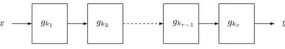
Iterated block cipher. Matsui’s Algorithm 2 [25] is a statistical cryptanalysis
method for finding a part of the last round key for an iterated block cipher. An iterated block cipher with block sizen bits processes plaintextx∈ {0,1}n and
expanded keyK0= (k1, k2, . . . , kr) by iterating a key-dependent round function
gk withk=ki,i= 1,2, . . . , r, to obtain ciphertexty, see Figure 1.
- - - -
-x gk1 gk2 gkr−1 gkr y
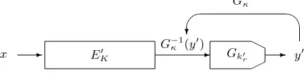
Last-round key-recovery attack. Key-recovery attacks on iterated block ciphers allow to recover information on the key-bits involved in one or more of the first rounds or last rounds, or both [4, 25]. To keep the notation simple, we restrict the description in this paper to key recovery attacks over the last round.
LetK0= (K, kr) denote the extended key, that is,K is the concatenation of
the keys k1, k2, . . . , kr−1. The first prerequisite for the last-round key recovery
attack is the so-called last round trick, which means that there is a part y0 of ciphertext y that can be computed from a part of the input to the last round and a part of the last round keykrusing a bijective function. Let us denote this
part ofkr bykr0 and the bijective function byGk0
r. Then it holds (see Figure 2) that
y0=Gk0 r(E
0
K(x)),
whereEK0 is the encryption function overr−1 rounds with its range restricted to the domain ofGk0
r.
H
-x EK0 - Gk0 - y0
r
G−1
κ
?
G−κ1(y0)
Fig. 2: Last round key recovery attack.
Then the attacker tries all possible key candidatesκofkr0. For the right key candidate κ=k0r it holds thatG−1
κ (y0) =EK0 (x), that is, the resulting data is
the same as obtained by encrypting plaintextxoverr−1 rounds of the cipher. The last round trick is not specific to linear cryptanalysis, but is often used also in the context of other statistical cryptanalysis, e.g., differential attacks. The important prerequisite for this type of attack is that the cipher has a statistical property that can be observed from the data obtained fromr−1 rounds of the cipher.
Correlation. The classical linear cryptanalysis exploits a biased linear
combi-nation of input and output bits over r−1 rounds of encryption EK0 . Given a vector u in the plaintext space and a vector v in the output space ofE0K the Boolean function u·x⊕v·EK0 (x) is called the linear approximation over EK0 with input maskuand output maskv, where “·” denotes the inner product. For example,u·xis themodulo2 sum of the coordinate-wise products of uandx. The strength of this linear approximation, also denoted as (u, v), is measured by its correlation defined as
cor(u, v)(K) =
2−nh#{x∈ {0,1}n|u·x+v·E0
K(x) = 0} −#{x∈F n
2|u·x+v·EK0 (x) = 1} i
Description of the attack. In the offline analysis of the cipher, the attacker selects a linear approximation (u, v) such that cor(u, v)(K) is large in absolute value, for all K. To launch an online attack, the cryptanalyst obtains a data sample from the cipher. We denote the data sample byD and the number of data items in D by N. In the case of classical linear cryptanalysis D is a set of plaintext-ciphertext pairs (x, y). From the ciphertext y only the part y0 is used in the attack.
Then the correct valuek0r is searched by trying all candidatesκand seeing if the cipher property, in this case large correlation, is observable from the data. To this end, the attacker obtains pairs (x, G−κ1(y0)), for all (x, y0) ∈ D, and
determines the empirical correlation
ˆ
c(D, K, kr, κ) =
2
N#{(x, y
0)∈D|u·x+v·G−1
κ (y0) = 0} −1.
After examining all candidates κ of k0
r, the cryptanalyst selects a set of
key-candidatesκthat achieve the top largest values|cˆ(D, K, kr, κ)|.
Success probability and advantage of the attack. It has become customary to
de-note by 2−a the proportion of keys that are discarded in this screening process
and call the exponent a the advantage of the attack [30]. On the other hand, the cryptanalyst must take care that the correct key kr0 is among the survived keys. Let us denote byPS the probability that the correct keykr0 survives. Then
PS is called the success probability of the attack. The value a can also
inter-preted as the number of key bits correctly determined by the screening process and therefore ais usually taken as a positive integer. Then the remaining key bits are determined by exhaustive search and the correct solution is found with probabilityPS. Clearly, there is a trade-off betweenaandPS. But more
impor-tantly, the larger |cor(u, v)(K)| is, the larger values aand PS can be achieved
by increasing the sample size N. The relationship between these quantities is established using a statistical model. In this section we provide the detail in the linear attack context.
(Distinct)-known plaintext attack. The statistical model depends also on the
way the cryptanalysts obtain the data sample. The pairs (x, y0) can be obtained by receiving them randomly, in which case, the attack is called known-plaintext (KP) attack. This can be modeled as pickingxrandomly and obtainingy0 for it. In statistical terms, we say that the sampling of (x, y0) is done with replacement.
2.2 Statistical Distributions
To estimate the data complexity of a statistical attack, we study the distribution of the random variables involved in the attack.
Let us denote byZ =Z(D, K, kr, κ) the random variable corresponding to
the number of solutions of the equationu·x+v·G−1
κ (y0) = 0, where (x, y0)∈D.
The n-bit block cipher with a fixed key K determines a probability p for a randomly selectedxto satisfy this equation. It is well known [18,25] that in case of KP sampling, the variable Z follows a binomial distribution with expected valueN pand varianceN p(1−p). In case of DKP sampling, by definition of the hypergeometric distribution, the variableZfollows a hypergeometric distribution with expected valueN pbut with variance
N p(1−p)2
n−N
2n−1,
which goes to zero as the sample size grows.
In this paper, we often consider KP and DKP alternatives within the same model. To this end, we introduce the following constantB which is defined by
B=
(1, for KP,
2n−N
2n−1, for DKP.
(1)
Both the binomial distribution and hypergeometric distribution allow tight ap-proximation using the normal distribution [33]. It means that a discrete random variable Z with binomial or hypergeometric distribution, whose all values are integers, is related to a continuous normal deviate X such that
Pr(Z =ζ)≈Pr(ζ−1
2 ≤X < ζ+ 1
2) (2)
In particular, the expected values and variances of Z and X are equal. In this paper, when we say that a discrete random variable follows a normal (or some other continuous) distribution, it is in the sense given in Equation (2). We then denote byZ ∼ N(µ, σ2) a random variableZwhich follows a normal distribution
with meanµand varianceσ2.
In the rest of this paper, the empirical correlation is interpreted as a discrete random variable. Due to the connection
ˆ
c(D, K, kr, κ) =
2
NZ(D, K, kr, κ)−1
and the normal approximation of the distribution ofZ(D, K, kr, κ), we say that
ˆ
c(D, K, kr, κ) follows a normal distribution with expected value
ExpD(ˆc(D, K, kr, κ)) = 2n−1#{x∈Fn2|u·x+v·G− 1
κ (y0) = 0} −1 = 2p−1
and variance
VarD(ˆc(D, K, kr, κ)) = ExpD(ˆc(D, K, kr, κ)2)−(ExpD(ˆc
2(D, K, k
r, κ)))2
= 1
whereB is defined as in Equation (1).
It should be noted that the approximation of the binomial distribution by a normal distribution is commonly accepted and has been verified experimentally in [1, 12, 18]. For more detailed considerations about distributions of discrete random variables arising from differential and linear cryptanalysis we refer to [18].
Later in this paper, we will also consider discrete random variables that are formed as a sum of squares of independent binomial variables. Since a sum of squares of independent standard normal deviates follows χ2 distribution, we will identify such a discrete random variable with a continuous χ2 distributed variable, and say that this discrete variable followsχ2 distribution.
The probabilitypdepends onK, kr and κ. The crucial distinction is made
between the cases κ=k0r and κ6=k0r. Previously also the dependency of pon
different values of κforκ6=k0
r has been studied [12]. This paper is the first to
present a statistical model of the behavior ofpin the caseκ=kr0 asK varies in the classical linear setting.
2.3 Statistical Hypothesis Testing
Given two random variablesTW andTR with respective cumulative distribution
functions FW and FR consider a situation that we have a value Θ, called a
threshold value, such that FW(Θ) > FR(Θ). Having observed a value T we
decide thatT is drawn from the distribution ofTRifT > Θ. IfT ≤Θwe decide
thatT is drawn from the distribution ofTW. Then error probabilities, the false
alarm ε0 and the non-detectionε1, are defined as
ε0= 1−FW(Θ) and ε1=FR(Θ).
The condition FW(Θ)> FR(Θ) guarantees that the probability that we reject
T when it is drawn fromTR is less than the probability that we acceptT when
it is drawn fromTW. ThenΘ=FW−1(1−ε0) =FR−1(ε1) and
ε1=FR(FW−1(1−ε0)). (4)
In the context of statistical cryptanalysis the cumulative distribution func-tions depend on the size N of the sample in such a way that, as N grows, Equation (4) is satisfied with smaller error probabilities 1−ε0 andε1. On the
other hand, given one error probability, the cryptanalyst can find an appropriate sample size and the other error probability to satisfy Equation (4), and then can compute a threshold value for the test.
In this paper, we will compute examples of this principle for normally dis-tributed test variables. Let us assume now thatTW andTRare normal deviates
with different means µW and µR. We consider w.l.o.g. the case µW < µR. Let
us denote the standard deviations σW andσR, respectively. Then we then have
ε0= 1−FW(Θ) = 1−Φ(Θ−σµW
W ) andε1=FR(Θ) =Φ(
Θ−µR
σR ), whereΦdenotes the cumulative distribution function of the standard normal distribution. From the symmetry of central normal distribution we get thatε1= 1−Φ(µRσ−Θ
Let us denote byζ0 andζ1the quantiles of the standard normal distribution
corresponding to the probabilities 1−ε0and 1−ε1. It means thatΦ(ζ0) = 1−ε0
and Φ(ζ1) = 1−ε1, where Φ denote the cumulative distribution function of
the standard normal distribution. Then we compute the threshold value Θ = µR−ζ1σR=µW +ζ0σW and by Equation (4) obtain
1−ε1=Φ(ζ1) =Φ
µ
R−µW −σWΦ−1(1−0)
σR
, (5)
which gives the success probability of TR, that is, the probability that decision
is correct when T is drawn from the distribution of TR. Such a threshold can
be found as soon as the standard deviationsσW andσRare sufficiently small to
satisfy
µW +σWζ0≤µR−σRζ1. (6)
The data complexity N is determined as the least sample size to obtain this inequality.
3
Classical Linear Key-Recovery Attack
3.1 Matsui’s Algorithm 2
A linear approximation (u, v) overEK0 consists of linear characteristics that are given as sequencesτ= (τ0=u, τ1, . . . , τr−2, τr−1=v) and its correlation can be
computed as a product of round-by-round correlation matrices [16]
c(u, v)(K) =X
τ r−1
Y
i=1
cor(τi−1·z+τi·gki(z)), (7)
where the sum is taken over all characteristics τ of the linear approximation (u, v).
The classical case of Matsui’s Algorithm 2 relies on the assumption that there exists a singleτ such that
c(u, v)(K)≈
r−1
Y
i=1
cor(τi−1·z+τi·gki(z))
for all keys K. Moreover, the original attack assumes that the block cipher is key-alternating, that is, the round function is of the formgk(z) =g(x⊕k). Then
a characteristic can be presented as follows
r−1
Y
i=1
cor(τi−1·z+τi·gki(z)) = (−1)
τ·Kρ τ,
Now we can formulate the assumptions about the statistical distributions of the empirical correlation for the wrong key and the right key. We restrict to the KP case for direct comparison with the previous treatments.
Let us denote by KW = (K, kr, κ) the key parameters that are used in
computing the empirical correlation ˆc(D, K, Kr, κ) for the wrong key candidate
κ 6= kr0, and denote in this case the counter by Z(D, KW) = Z(D, K, Kr, κ)
the empirical correlation by ˆc(D, KW) = ˆc(D, K, Kr, κ). Since the data is not
obtained from the cipher, it is not expected to exhibit the bias of the linear approximation. Specifically, it is assumed that for a given keyKW, the counter
Z(D, KW) is binomially distributed with p= 1/2, which leads to the following
assumption about the continuous approximation of this probability distribution.
Wrong-key randomization hypothesis: For a wrong key candidate, ˆc(D, KW)
fol-lows normal distribution with parameters
ExpD(ˆc(D, KW)) = 0
VarD(ˆc(D, KW)) =
1 N.
In a similar way, let us denote by KR = (K, kr, κ) when κ = kr0, and
de-note byZ(D, KR) =Z(D, K, Kr, κ) the counter and by ˆc(D, KR) the empirical
correlation in this case. Note that following the notation of Section 2.1 we have
ˆ
c(D, KR) =
2
N#{x∈D|u·x+v·E
0
K = 0} −1
which is independent of the value of kr and κ = kr0. The expected value of
ˆ
c(D, KR) taken over data D is then the correlation c(u, v)(K) of the linear
approximation, which for each key K is assumed to be equal toc or −c in this classical case of a single dominant characteristic. This leads to the following assumption.
Hypothesis of right-key equivalence: For all correct key κ = kr0 the empirical
correlation ˆc(D, KR) follows normal distribution with parameters
ExpD(ˆc(D, KR)) =±c
VarD(ˆc(D, KR)) = ExpD
(ˆc(D, KR)−ExpD(ˆc(D, KR)))
2
= 1 N(1−c
2).
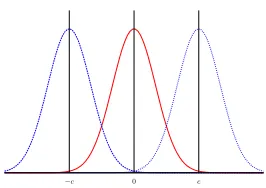
Here it is usually estimated 1−c2≈1. Under these assumptions there are three
normal distributions as depicted in Figure 3. In any practical instance with a fixed encryption key (K, kr), only two of the distributions are present, the middle
distribution and exactly one of the other two, but the cryptanalyst does not know which of the two. It implies that wrong keys will be accepted on both sides.
When testing the key candidates, the cryptanalyst is facing with the task of statistical hypothesis testing: given the value |ˆc(D, K, kr, κ)|computed from
0
−c c
Fig. 3: Three normal distributions related to classical linear key-recovery attack: middle curve = wrong keyKW with ExpD(ˆc(D, KW)) = 0
left curve = right keyKRwith ExpD(ˆc(D, KR)) =−c right curve = right keyKR with ExpD(ˆc(D, KR)) =c
last-round keyκ=kr0, or if it is not from the cipher, and the key candidateκis
rejected.
Let us now apply the hypothesis testing paradigm explained in Section 2.3 to the key recovery attack. LetTW be the observed correlation computed with the
wrong key candidate and TR the observed correlation with the right key. Then
µW = 0 andµR=c, and σW2 = 1/N andσ2R= 1/N(1−c2).
Let us denote the error probabilities
α0= 2−a andα1= 1−PS,
whereα0is the probability that a wrong key candidate is accepted andα1is the
probability that the correct key is rejected. Since wrong keys can be accepted on both sides, the error probabilities for the test are
ε0=
1 2α0= 2
−(a+1) andε
1=α1= 1−PS.
By substituting these values to Equation (5) we can solve for data complexity boundN and thresholdΘsuch thatΘ=p1/N ζ0=c−
p
(1−c2)/N ζ 1 and
PS=Φ(ζ1) =Φ
c−ϕa+1
p
1/N
p
(1−c2)/N
!
, (8)
where we have denoted the quantiles as ζ0 = Φ−1(1−2−(a+1)) = ϕa+1 and
ζ1=Φ−1(PS) =ϕPS.
The case ExpD(ˆc(D, KR))<0 is a mirror image of the case explained above
and −Θ can be taken as a threshold will be−Θ. Then the key candidate κis accepted if ˆc(D, K, kr, κ)> Θ or ˆc(D, K, kr, κ)<−Θ and rejected otherwise.
Let us summarize the derivations in the following theorem, which is a refine-ment of the original result of Matsui [25]. The same formula (assuming 1−c2≈1)
Theorem 1. Assume that anr-round block cipher has a linear approximation
with a single dominant characteristic over r−1 rounds and correlation with
absolute value about equal to c. Assume that the hypotheses of right-key
equiva-lence and wrong-key randomization hold. Then the key-recovery attack presented
in this section will succeed with probabilityPS and advantagea if the size N of
the available data sample satisfies
N ≥(ϕa+1+ √
1−c2ϕ
PS)
2
c2 .
3.2 Integrating Key Variable in the Model
Only recently, the hypothesis of right-key equivalence and the wrong-key ran-domization hypothesis have been questioned, as it has been observed in practical experiments that the statistical distributions may vary significantly as the key varies. The same holds for the wrong key case. For each wrong key candidate the statistical distribution of ˆc(D, KW) is different. Strong evidence was brought
up that it is not accurate to model wrong keys to draw test statistic from the uniform distribution [12, 26].
The wrong key case. In [12] the distribution of the empirical correlation ˆc(D, KW)
was examined in the case of a wrong keyKW. Specifically, it was noted that the
empirical correlation depends on two mutually independent random variables KW andD. Letκ6=kr0, and denote
˜
c(KW) = ˜c(K, kr, κ) = 2n−1#{x∈Fn2|u·x+v·G
−1
κ (y
0) = 0} −1
= ExpD(ˆc(D, KW)).
In other words, ˜c(KW) is the correlation of the linear approximation (u, v)
com-puted over the function G−1
κ ◦Gk0
r ◦E
0
K. The original wrong-key
randomiza-tion hypothesis assumed that these correlarandomiza-tions are equal for all wrong keys KW = (K, kr, κ). Based on the remark after Corollary 4.3 of [18], in [12] they
suggested to revise the wrong-key randomization hypothesis as follows.
Hypothesis 1 Revised wrong-key randomization hypothesis: For each wrong key
KW = (K, kr, κ), the function G−κ1◦Gk0 r ◦E
0
K is a random vectorial Boolean
function and the correlation of its linear approximation has the following distri-bution
˜
c(KW)∼ N(0,2−n).
Based on this hypothesis the following result was stated in [12] but the proof was omitted. We give also the proof here.
Theorem 2. Suppose that the revised wrong-key randomization hypothesis holds for anr-round block cipher. Then the empirical correlationcˆ(D, KW)is
approx-imately normally distributed with parameters
ExpD,KW(ˆc(D, KW)) = 0 and VarD,KW(ˆc(D, KW)) = 1 N + 2
Proof. The aim is to determine the distribution of ˆc(D, KW) when bothD and
K are simultaneously taken into consideration as random variables. We write ˆ
c(D, KW) as a sum of two random variables
(ˆc(D, KW)−˜c(KW)) + ˜c(KW), (10)
where, for each fixedKW,
ˆ
c(D, KW)−c˜(KW)∼ N(0,
1
N(1−˜c(KW)
2)).
We observe that 2nc˜(KW)2∼χ2 with one degree of freedom and has the mean
2−nand variance 21−2n. Hence it is negligible and often omitted in similar deriva-tions, see e.g. [30], by replacing the true variance of the first variable by a key-independent upper-bound 1
N. Then we apply the revised wrong-key
randomiza-tion hypothesis to the second part of Equarandomiza-tion (10), which is independent ofD, to obtain that ˆc(D, KW) can be expressed as a sum of two independent normally
distributed variables, the first one ˆc(D, KW)−˜c(KW)∼ N(0,N1) depending on
D only, and the second one ˜c(KW)∼ N(0,2−n) depending onKW. ut
The right key case. Next we complete the statistical model of the classical linear
attack by making the corresponding adjustment to the variance of the empirical correlation in the right key case. Let us start by recalling the Linear hull theorem for iterated block ciphers. The proof of this classical result was given in [28]. The special case of key-alternating cipher was considered and proven in [17]. It is interesting to note that the Linear hull theorem, stated for a general Boolean function, has found applications also in coding theory [15] and in the theory of Boolean complexity [24].
Theorem 3. Let (u, v) be a linear approximation and denote c(u, v)(K) = cor(u·x+v ·E0
K(x)) and c(u, τ, v) = cor(u·x+τ ·K +c ·EK0 (x)). Then
the average of c(u, v)(K)2 taken over K is equal to the sum of c(u, τ, v)2 taken overτ.
Note thatc(u, v)(K) is computed as the correlation over the space of the plain-text x with a fixed key K, while correlation c(u, τ, v) is computed over the plaintextxand the keyK. The latter is also called the correlation of the char-acteristicsτ. Let|K|denote the length ofK in bits. The quantity
2−|K|X
K
c(u, v)(K)2=X
τ
c(u, τ, v)2
where the sum on right side is taken over all characteristics τ of the linear approximation (u, v) is called the expected linear potential of (u, v) and denoted asELP(u, v) or justELP if the linear approximation is clear from the context. Matsui’s Algorithm 2 assumes a single characteristic τ with a dominating correlation, which takes the form (−1)τ·Kρ
whichτ·K= 0 and byK1the keys for which τ·K= 1. Then the assumption
about dominating characteristic can be formalized as follows
ExpK∈K0(c(u, v)(K)) =ρτ and ExpK∈K1c(u, v)(K) =−ρτ.
So the expected values of the correlations taken over the the two disjoint halfs of the keyspace are±c. Moreover, it is natural to assume that the variances of c(u, v)(K) over the two disjoint halfs of the keyspace are equal, that is,
ExpK∈K0(c(u, v)(K)2)−c2= ExpK∈K1(c(u, v)(K)2)−c2,
in which case
ExpK∈K
0(c(u, v)(K)
2) = Exp
K∈K1(c(u, v)(K)
2)
= ExpK(c(u, v)(K)
2
) =ELP(u, v).
It follows that
VarK∈K0(c(u, v)(K)) = VarK∈K1(c(u, v)(K)) = X
t6=τ
c(u, t, v)2=ELP−c2.
Let us state this property, which was derived under specific assumptions, as a following hypothesis.
Hypothesis 2 Revised hypothesis of right-key equivalence: When the keyK is
taken as a random variable over the half space K0 or K1, the correlations are
distributed as follows
c(u, v)(K)∼ N(±c, ELP−c2),
where the mean is positive for one half space and negative for the other.
Theorem 4. In the context of a linear key-recovery attack of an iterated block cipher described in this section, the empirical correlationˆc(D, KR)approximately
follows exactly one of the two normal distributions with parameters
ExpD,K(ˆc(D, KR)) =±c and VarD,K(ˆc(D, KR)) =
1
N +ELP −c
2.(11)
The choice between these distribution happens with probability equal to one half.
Proof. The proof is similar to the one in the wrong key case. Assuming that these
two probability distributions can be approximated by a normal distribution, we can write ˆc(D, KR) as a sum of two normal deviates
(ˆc(D, KR)−c(u, v)(K)) +c(u, v)(K)
For each fixed keyKR, the first term is a normal deviate of the random variable
D with mean 0 and variance 1
N(1−c(u, v)(K)
2). Replacing 1
N(1−c(u, v)
2) by
its close upper bound 1
N, we obtain that (ˆc(D, KR)−c(u, v)(K))∼N(0,
1
N) and
is independent of K. The distribution of the second term can be approximated with exactly one of two normal distributionsN(c, ELP−c2) orN(−c, ELP−c2)
By substituting the adjusted variances to the formula of the success proba-bility given in Equation (8) we get
PS ≈Φ
c√N−ϕa+1 √
1 +N2−nϕ
a+1
p
1 +N(ELP−c2)
!
.
IfELP =c2 for all encryption keys as assumed by the Hypothesis of right-key equivalence, then this formula is identical to Equation (6) in [12].
In reality, it would be more accurate to assume the value
ELP−c2=X
t6=τ
c(u, τ, v)2
to be bounded from below by the variance of random noise which is equal to 2−n. If the equality can be assumed to hold, that is, the linear approximation
is composed of one linear characteristic and pure noise, then by takingELP = c2+ 2−n we obtain the following complexity bound for the KP sampling in
Matsui’s Algorithm 2
N ≥ (ϕa+1+ϕPS) 2
c2−2−n(ϕ
a+1+ϕPS)
2.
This complexity bound is larger than the one given in Theorem 1 due to the variance over the key, and gives meaningful values forc >2−n/2(ϕ
a+1+ϕPS).
3.3 Several Dominant Characteristics
If the number of dominant characteristics is small, the approach of single dom-inant characteristic discussed in the previous section can be applied and the key space will be divided into 2d parts according to the expected value of the
correlation. This approach was taken in [29] where it was shown that it is possi-ble to distinguish between different values of correlations up to seven rounds of PRESENT. As the number of dominant characteristics grows, the correlation as expressed in Equation (7) will take several different values with non-negligible absolute value and it becomes unfeasible to distinguish between them. Moreover, this often means that for an increasing number of encryption keys the correlation will be equal, or close, to zero. Most modern ciphers have been designed like this to avoid linear cryptanalysis. Then the key space cannot be partitioned as in the classical Matsui’s Algorithm 2, but instead, it is considered as a whole. Conse-quently, the expected value of the empirical correlation, now taken over all keys, is typically close to zero. Indeed, it is very likely that the average correlation is equal to zero. This situation is interpreted by Daemen and Rijmen [18] as fol-lows: “The average correlation of a hull gives no indication about the complexity of a linear attack. Therefore, we only talk about the ELP of a hull.” Next we elaborate what this means in practice.
we denote by σ2. Moreover, we assume normal distribution as state it as the
following.
Hypothesis 3 Right-key randomization hypothesis: The correlations of a block
cipher are random variables of keyK and follow normal distribution
c(u, v)(K)∼ N(c, ELP−c2).
We now state the following theorem. This theorem is the basic building block of the new statistical model of multiple linear cryptanalysis. Therefore we include both KP and DKP cases of data sampling in this theorem.
Theorem 5. Assume that the Right-key randomization hypothesis holds. Then the empirical correlation ˆc(D, KR) of (u, v) is a normally distributed random
variable of D andK and
ExpD,K(ˆc(D, KR)) =c and VarD,K(ˆc(D, KR)) =
B
N +ELP−c
2, (12)
whereB is defined depending of the sampling in Equation (1).
Proof. The claim follows by splitting the random variable ˆc(D, KR) to two parts
(ˆc(D, KR)−c(u, v)(K)) +c(u, v)(K).
Similarly, as in the case of a single dominant characteristic, the probability dis-tribution of the first part can be approximated by a normal deviate which is independent of the key variableK. It has expected value equal to zero and vari-ance equal to BN. By assumption, the second part is a normal deviate of the random variable K. Then the probability distribution of ˆc(D, KR) can be
ap-proximated by a sum of two independent normal deviates which has the claimed
parameters. ut
The form of the probability distribution ofc(u, v)(K) has been seen normal for many practical ciphers [1]. One example is the cipher PRESENT [10], for which, in addition, the expected valuesc of correlations are practically equal to zero. In such a case the means of the empirical correlations in the wrong and right key cases are the same, that is, equal to zero. But the variances are different which makes distinguishing possible also in this case. By Theorem 2 the variance in the wrong key case is equal to 2−n which is less than ELP. The approach
is to use the square ˆc(D, K, kr, κ)2 as a test statistic, which in both cases is
a constant multiple of a χ2-distributed random variable where the constant is
equal to NB +ELP in the right key case and BN + 2−n in the wrong key case.
Hence the test statistic has different means BN +ELP or BN+ 2−n and variances 2(B
N +ELP)
2or 2(B
N + 2
−n)2in the right key and wrong key case, respectively.
in variances can be amplified even further and the distinguisher improved. This approach was first modeled in [6] by assuming that the involved linear approxi-mations are independent. This model covered the statistics as a random variable over the data sample and assumed that the behavior is practically the same for all keys. Similarly, the extension of the statistical model to multidimensional linear cryptanalysis presented in [19] did not take into account the effect of the key. The goal of the next section is to complete these models and include the key variable to them.
4
Multiple and Multidimensional Linear Attacks
4.1 Capacity
In [6] the statistical model of taking advantage of multiple independent linear approximations in key-recovery attacks was presented. In the more recent mul-tidimensional linear attacks introduced in [19], the attacker exploits of all linear approximations with linear masks (u, v)6= 0 in a linear space. The main benefit of the latter approach is that it does not require the assumption of independence of the linear approximations.
The main motivation and challenges of the work presented in this section originate from the multidimensional linear attack, but due to the generic link between linear and differential types of attacks [7], the results can also be applied to truncated differential attacks.
To collect information of the correlations of all the linear approximations over EK0 used in the attack, the notion of capacity was introduced in [6] and generalized in [19]. Given a set of input and output linear mask pairs (uj, vj),
j = 1, . . . , `, where (uj, vj) 6= 0, their capacity is defined as the sum of the
squared correlations:
C(K) =
` X
j=1
c(uj, vj)(K)2. (13)
In case the linear approximations (uj, vj) form the set of non-zero elements of
a linear spaceU×V of dimensions, that is, `+ 1 = 2s, then the capacity can
also be computed as
C(K) = 2s
` X
η=0
pη(K)−2−s 2
, (14)
wherepη(K) is the probability that a data value (x, EK0 (x)) restricted toU×V
takes the value η ∈ U ×V. In other words, C(K) is the squared Euclidean imbalance [3] of the probability distributionpη(K).
structures such as Feistel-type ciphers. When multiple approximations with zero-correlation are used, the capacity C(K) of the set of linear approximations is equal to zero for all keysK.
To capture the statistical behavior of capacities we develop a model that takes also the key variance into account. The case of wrong keys is straightforward as all empirical correlations are independently and identically distributed as D and KW varies. The right key case requires some additional assumptions.
In [20], the cipher correlations were assumed independent and certain weak key quantiles where determined and tested for multiple linear key recovery attack on the PRESENT cipher.
4.2 Key-Recovery Attack
We consider the same last-round key-recovery setting as in Section 2. In (zero-correlation) multiple/multidimensional linear key-recovery attacks the test statis-tic is the empirical capacity of a set of linear approximations. We denote it by T(D, K, kr, κ) and it is computed as follows
T =T(D, K, kr, κ) =N ` X
j=1
ˆ
cj(D, K, kr, κ)2, (15)
where ˆcj(D, K, kr, κ) is the empirical correlation of thej-th linear approximation
uj·x+vj·Gκ−1(EK0(x)).
In multidimensional linear key-recovery attacks, the online test statistic is computed over all non-zero linear approximations, in which case, instead of the individual empirical correlations, cryptanalyst may compute the test statistic over the observed data (x, G−1
κ (y0)),x∈U andGκ−1(y0)∈V, also as follows
T =T(D, K, kr, κ) = ` X
η=0
(V[η]−N2−s)2
N2−s , (16)
where V[η] corresponds to the number of occurrences of the value η of the observed data distribution. In the offline analysis, only a subset of all linear approximations in a linear space U ×V are taken into consideration when the capacity estimate is computed.
In the following, we study the statistical distributions of multiple and multi-dimensional linear cryptanalysis as the encryption key and the wrong key candi-dates vary and provide new key-dependent distribution parameters. With these new developments we aim at improving the estimate of the data complexity. One of the main obstacles that still remains is how to estimate the variance of T(D, K, kr, κ) for κ=kr0. We will also present some approaches how to tackle
this problem.
4.3 Statistical Model for the Wrong Keys
in Section 3.2 holds. As shown in Theorem 2 and the remark after it, the em-pirical correlation ˆc(D, KW), KW = (K, kr, κ), whereκ6=k0r, is approximately
normally distributed with parameters
ExpD,KW(ˆc(D, KW)) = 0 and VarD,KW(ˆc(D, KW)) = 1 NB+ 2
−n,
where the constantB is determined as in Equation (1) according to KP or DKP sampling.
Let us denote the number of exploited linear approximations by`. Then we can write the test statistic computed for wrong keyKW in multiple or
multidi-mensional linear key recovery attack as follows
T =T(D, KW) =N ` X
j=1
ˆ
cj(D, KW)2= (B+ 2−nN) ` X
j=1
ˆ
cj(D, KW)2
1
NB+ 2−
n .
Note that qcˆj(D, KW)
1
NB+ 2−
n
∼ N(0,1). As for a random function, the linear
approx-imations are independent, it follows that
T
B+ 2−nN ∼χ
2
` (17)
and the parameters of the probability distribution of T are as given by the following theorem.
Theorem 6. Assuming that the revised wrong-key hypothesis holds for` linear approximations involved in a multiple or multidimensional linear attack, then
the statistic T(D, KW) computed as in Equation (15) (or Equation (16)) is a
constant multiple of a χ2-distributed variable with` degrees of freedom and has
the following mean and variance
ExpD,KW(T(D, KW)) =B`+N2−n` and (18)
VarD,KW(T(D, KW)) = 2
` B`+N2
−n`2
,
whereB is defined as in Equation (1).
Proof. From Equation (17) and by definition of theχ2distribution, we have
ExpD,KW
T
B+ 2−nN
=`
and
VarD,KW
T
B+ 2−nN
= 2`.
We highlight the following special case and state it as a separate corollary.
Corollary 1. In the context of Theorem 6 suppose that sampling is done using
distinct known plaintexts. Then the statisticT(D, KW)has the following mean
and variance
ExpD,K
W(T(D, KW))≈` VarD,KW(T(D, KW))≈2`.
Proof. By substituting B = (2n −N)/(2n −1) to Equation (18) we get the
result. ut
Interestingly, these are exactly the parameters that have been used in previous works to model the wrong-key distribution for DKP sampling in multidimen-sional zero-correlation attacks in [9, 11]. However, no justification of these pa-rameter values can be found in the previous literature. As KP sampling from a uniform distribution will yield the same distribution parameters for T(D, KW),
it is possible that those parameters have been reused in DKP case in the lack of anything better. Fortunately, the parameter values were correct and the existing zero-correlation attacks that use DKP remain correct.
The situation is not that fortunate for general multidimensional linear attacks that use KP. The data complexity estimate as given in Equation (21) has been derived under the hypothesis that the wrong-key data is drawn from the uniform distribution with ExpD,KW(T(D, KW)) = ` and VarD,KW(T(D, KW)) = 2`, see Equation (17) of [19]. This is certainly too optimistic for the attacker, since the data distributions in multidimensional linear approximation in ran-dom case are unlikely to become completely uniform. The more realistic values of parameters in the KP case are ExpD,KW(T(D, KW)) = `(1 +N2
−n) and
VarD,KW(T(D, KW)) = 2`(1 +N2
−n)2 as given by our analysis in Theorem 6.
Remark 1. We denote byC(KW) =P
`
j=1c˜j(KW)2with ˜cj(KW) = ˜c(K, kr, κ) =
2n−1#{x∈
Fn2|uj·x+vj·G−κ1(y0) = 0} −1 the capacity for a given wrong key.
Assuming the Revised wrong-key randomization hypothesis, we havecj(KW)∼
N(0,2−n) and by definition, a constant multiplier of C(KW) follows a χ2
dis-tribution with ` degrees of freedom. It means that C(KW) follows a gamma
distribution with ExpKW(C(KW)) =`/2
n and Var
KW(C(KW)) = 2 1−2n`.
4.4 Modeling the Right Key Behavior
In Section 3.3, we gave the distribution of correlation of a single linear approxi-mation (see Theorem 5). In this section we model the behavior of the statisticT involved in a multiple/multidimensional linear attack for the right key using the same straightforward approach as in the wrong-key case presented above. The result is obtained by combining the squares of normally distributed correlations into a (constant multiple of) aχ2distributed statistic. This is basically how the
distributions ofT(D, KR), for the right keyKR= (K, kr, κ), whereκ=kr0, were
Hypothesis 4 (Key-variance hypothesis – multiple:) The empirical correlations
ˆ
cj(D, KR),j= 1,2,· · ·, `of the multiple linear approximations involved in
Equa-tion (15) are statistically independent and their expected values cor(uj, vj)(K)
taken over the data are normal deviates of K and have equal variances.
For the sake of clarity, let us introduce the following notations before present-ing the result. Given 1≤j ≤`, the correlations of the`linear approximations are, for a fixed key K, denoted by cj(K) = cor(uj, vj)(K) = ExpD(ˆcj(D, KR))
andcj= ExpK(cj(K)). Given the expected linear potentialsELPj=ELP(uj, vj)
as defined in Section 3.2, the capacity is
C= ExpK(C(K)) =
` X
j=1
ExpK(cj(K)2) = ` X
j=1
ELPj.
Since in general ExpK(cj(K)2)6= ExpK(cj(K))2, we also introduceC0=P
`
j=1c
2
j
which can be interpreted as the capacity of the expected correlations. We then state the following result.
Theorem 7. Suppose that the linear approximations involved in the computa-tion of the attack statistic as in Equacomputa-tion (15)
T =T(D, KR) = ` X
j=1
ˆ
cj(D, KR)2
satisfy Hypotheses 2 and 4. We have
Q= T
B+N`(C−C0)
∼χ2`(δ),
where the non-centrality parameter of theχ2 distribution is
δ= N C0 B+N`(C−C0)
,
andB is defined as in Equation (1).
Proof. By Hypotheses 2 and 4 we can apply Theorem 5 for eachj = 1,2, . . . , `
and get that each ˆcj(D, KR) follows normal distribution with parameters
ExpD,Kˆcj(D, KR) =cj and VarD,Kˆcj(D, KR) =
B
N +ELPj−c
2
j,
and moreover, they are all independent.
With the notations previously defined, the summation overj gives
` X
j=1
VarD,K(ˆcj(D, KR)) =
B
It then follows by Hypothesis 4 that
VarD,K(ˆcj(D, KR)) =
B N +
C−C0
` .
Moreover, by Hypothesis 4 the empirical correlations are normal deviates, mean-ing that for allj,
ˆ
cj(D, KR) q
B
N +
C−C0
` ∼ N cj q B N +
C−C0
`
,1
.
By definition of the non-centralχ2 distribution we obtain that
Q= T
B+N`(C−C0)
= ` X j=1 ˆ
cj(D, KR) q
B
N +
C−C0
`
2
follows a non-central χ2 distribution with`degrees of freedom and non-central
parameter δ= ` X j=1 cj q B N +
C−C0
`
.
u t
Let us recall that in the multidimensional case, when the keyKis fixed and the statistic T is computed by Equation (16) over 2s data valuesη, the empirical frequencies V[η] are independent random variables of D for all but one η, for which V[η] is determined by the other values. Therefore, we only need an as-sumption about their expected values pη(K) to prove Theorem 7 in this case.
This assumption is formulated as follows, where we recall thatP`
η=0pη= 1 and
therefore, for eachK, only`of the valuespη(K) can be taken as free variables.
Hypothesis 5 (Key-variance hypothesis – multidimensional:) For each fixed data valueη= 0, . . . ,2s−1, the probabilitiesp
η(K)taken as random variables of
K, are normal deviates with equal variances. Moreover, each subset of ` values
pη(K)are independent, and they determine the remaining value uniquely.
Under the previous hypothesis we obtain the following result which is similar to the one of Theorem 7.
Theorem 8. Suppose that the expected valuespη(K) = ExpD(V[η]/N)involved
in the computation of the attack statistic as in Equation (16)
T =T(D, K, kr, κ) = ` X
η=0
(V[η]−N2−s)2
satisfy Hypothesis 5. Then
Q= T
B+N`(C−C0)
∼χ2`(δ),
where the non-centrality parameter of theχ2 distribution is
δ= N C0 B+N`(C−C0)
,
andB is defined as in Equation (1).
Proof. Let us start by computing the sum of the variances of pη(K) over η =
0,1,2, . . . , `= 2s−1. We obtain
` X
η=0
VarKpη(K) = ` X
η=0
ExpK(pη(K)2)−p2η
= 2−s(C+ 1)−2−s(C0+ 1) =
C−C0
`+ 1 .
Without loss of generality, we denote byp0(K) the probability that is determined
by the other probabilities.pη(K),η6= 0. Then by Hypothesis 5
pη(K)∼ N
pη,
C−C0
`(`+ 1)
, η6= 0.
It follows that
N pη(K)∼ N
N pη, N2
C−C0
`(`+ 1)
, η6= 0.
On the other hand, for each fixedK, the frequencyV[η],η6= 0 follows a binomial distribution with probability pη(K). We estimate pη(K)(1−pη(K)) ≈2−s as
usual. Then
V[η]−N pη(K)∼ N(0, BN2−s), η6= 0,
and this distribution is independent of K, and hence, independent ofN pη(K) .
It follows that
V[η]∼ N
N pη,
N `+ 1(B+
N
`(C−C0)
.
The rest of the proof is analogical to the proof of Theorem 7. ut
The distribution of T = T(D, KR). Summarizing the results of Theorems 7
and 8, the test statisticT has the following parameters
ExpD,K(T(D, KR)) = (`+δ)(B+
N
` (C−C0) =B`+N C
VarD,K(T(D, KR)) = 2(`+ 2δ)(B+
N
` (C−C0)
2 (19)
=2
`((`+δ)
2−δ2))(B+N
` (C−C0)
2
=2
`((B`+N C)
The form of the distribution ofT can be determined in two cases:
1. ` >50, in which case normal approximation can be used, or 2. C0= 0, in which caseT follows a gamma distribution
T(D, KR)∼Γ `
2,2(B+N C
`)
.
Both of these cases are important for applications.
In the next section, we present results of our experiments when` >50 and C0= 0. In particular we compare the theoretical estimates of the mean and the
variance from Equation (19) with the experimental ones.
In the experiments we use versions of the SMALLPRESENT cipher where we can compute the correlations and capacities for the full codebook. In practical applications, however, the problem of how to obtain accurate estimates of the expected values and variances of the test statistics which are needed to estimate the data complexity of the key recovery attack. This question, as well as testing the accuracy of Hypotheses 4 and 5 require cipher specific information. We have investigated the case of the key-alternating block cipher and will present the results of this work in a forthcoming paper.
⊕ ⊕ ⊕ ⊕ ⊕ ⊕ ⊕ ⊕ ⊕ ⊕ ⊕ ⊕ ⊕ ⊕ ⊕ ⊕ ⊕ ⊕ ⊕ ⊕ ⊕ ⊕ ⊕ ⊕ ⊕ ⊕ ⊕ ⊕ ⊕ ⊕ ⊕ ⊕
S7 S6 S5 S4 S3 S2 S1 S0
⊕ ⊕ ⊕ ⊕ ⊕ ⊕ ⊕ ⊕ ⊕ ⊕ ⊕ ⊕ ⊕ ⊕ ⊕ ⊕
S3 S2 S1 S0
4.5 Experiments on SMALLPRESENT
In this section, we verify developed theory by comparing the experimental and theoretical mean ExpD,K(T(D, KR)) of the test statisticT in the cases of DKP
and KP sampling.
The experiments have been conducted on two scale versions [22] of the block cipher PRESENT [10]. SMALLPRESENT-[8] is a 32-bit cipher designed with the 80-bit original key-schedule of PRESENT. SMALLPRESENT-[4] is a 16-bit cipher. The round functions of both ciphers are depicted in Figure 4. For the experiments on SMALLPRESENT-[4], a 20-bit key-schedule has been defined. The multidimensional distributions are respectively involving`= 255 and`= 63 linear approximations.
In all cases the capacity of the multidimensional approximation used in the theoretical models is the true value determined from the cipher.
In Figures 5 and 6, we compare the theoretical means given by Equation (19) of statisticT with the experimental ones for both distinct and non-distinct plain-text. For this cipher, the values seem to match very well.
6 6.5 7 7.5 8
12 12.5 13 13.5 14 14.5 15 15.5 16
log
2
(Exp
D
,K
(
T
(
D
,K
R
)))
log2(N)
`(1−N/2n) +N C Experimental DKP
`+N C
Experimental KP
Fig. 5: The mean ExpD,K(T(D, KR)) for a 6-bit multidimensional distribution (` = 26−1) over 4 rounds of SMALLPRESENT-[4] with capacityC= 2−9.20.
In Figures 7 and 8, the corresponding variances are analyzed. We observe that the theoretical value is significantly improved when the key variance is taken into account. Still there is in all cases a clear gap between the theoretical value VarD,K(T(D, KR)) given by Equation (19) and the experimental values of
the variance.
In the computation of the theoretical value`is taken equal to 2s−1 wheres
8.5 9 9.5 10 10.5
26 27 28 29 30 31 32
log
2
(Exp
D
,K
(
T
(
D
,K
R
)))
log2(N)
`(1−N/2n) +N C Experimental DKP
`+N C
Experimental KP
Fig. 6: The mean ExpD,K(T(D, KR)) for a 8-bit multidimensional distribution (` = 28−1) over 9 rounds of SMALLPRESENT-[8] with capacityC= 2−21.29.
only small deviation from it was observed in simulations on these SMALLPRE-SENT variants. On the other hand, it is known that due to the linear properties of the S-box, PRESENT ciphers allow accurate estimation of the capacity using single-bit linear characteristics that can be considered statistically independent. Therefore also the alternative approach of multiple independent linear approxi-mations, that is, the use of Hypothesis 4 would be justified.
Let us examine these alternative approaches in the case of SMALLPRESENT-[8]. The observed multidimensional linear approximation consists of 4 bits of in-put to one S-box and 4 bits outin-put of one S-box after 9 rounds. If Hypothesis 5 is applied, we take`= 28−1. By this approach we get an underestimate of the
variance of T(D, KR) which is depicted in Figure 8. An alternative approach
could be to include only the most dominant linear characteristics between these S-boxes, that is, by taking all single-bit characteristics leading from the three leftmost bits from the output of first S-box to the three leftmost bits of the input to the last S-box. This approach, however, seems in our experiments to give an overestimate of the variance ofT(D, KR). The true value lies between these two
extremes. Closing this gap and obtaining more accurate estimate of the variance is left for future work.
5
Data Complexity
5.1 Previous Model
The multidimensional linear cryptanalysis [19] traditionally assumes known plain-text and that the cryptanalyst does not have any means to check for repetitions in the plaintext. Then the statisticT given in Equation (16) computed from the multidimensional distribution for a fixed key (K, kr, κ) follows, up to a constant
multiplier, aχ2 distribution both forκ=k0
7 8 9 10 11 12 13
12 12.5 13 13.5 14 14.5 15 15.5 16
log
2
(V
ar
D
,K
(
T
(
D
,K
R
)))
log2(N)
2`(1−N/2n) + 4N C 2
`(`(1−N/2 n) +N C)2 Experimental DKP 2`+ 4N C
2 `(`+N C)
2
Experimental KP
Fig. 7: The variance VarD,K(T(D, KR)) for a 6-bit multidimensional distribution (`= 26−1) over 4 rounds of SMALLPRESENT-[4] with capacityC= 2−9.20.
KP model given in [19] were the following:
Exp(T(D, KR))≈`+N·C and Var(T(D, KR))≈2(`+ 2·N·C),
Exp(T(D, KW))≈` and Var(T(D, KW))≈2`.
(20)
The distributions for wrong and right key candidates have different means and variances and thus it is possible to distinguish between them by statistical inference analogical to the hypothesis testing method described in Section 3.1 but this time between two χ2 distributed random variables. Then the error probabilities and the corresponding quantiles by replacing the cumulative density function Φ by the cumulative density function of the χ2 distribution with `
degrees of freedom.
In practice, it is accurate to approximateχ2distributions using normal
distri-bution as soon as`= 2s−1>50. Using the parameters given by Equation (20),
and by denoting the advantage and success probability of the key-recovery at-tack respectively byaandPS, the following estimate of the data complexity of
a KP multidimensional linear attack was given in [19]
N ≈ √
4a`+ 4Φ−1(2P
S−1)2
C . (21)
9 10 11 12 13 14 15 16 17 18
26 27 28 29 30 31 32
log 2 (V ar D ,K ( T ( D ,K R )))
log2(N)
2`(1−N/2n) + 4N C 2
`(`(1−N/2 n) +N C)2 Experimental DKP 2`+ 4N C
2 `(`+N C)
2
Experimental KP
Fig. 8: The variance VarD,K(T(D, KR)) for a 8-bit multidimensional distribution (`= 28−1) over 9 rounds of SMALLPRESENT-[8] with capacityC= 2−21.29.
5.2 Data Complexity Estimates
In the hypothesis testing context described in Section 2.3, we can estimate the data complexity of a multiple/multidimensional linear attack. In this section, since we do not yet know how to estimate the value ofC0, we assume thatC0= 0.
As explained at the end of Section 4.4, this means that the random variable T(D, KR) follows a gamma distribution. Using Equation (4) we could therefore
obtain an accurate formula of the success probability of the attack. However in order to compare with previous works we assume that` >50, which is the case in most attacks, and use normal approximations of the gamma distributions of T(D, KW) and T(D, KR). We denote by CR = ExpK(C(K)) and CW =
ExpKW(C(KW)) the expected values of the capacity for respectively the right
and wrong keys.
Corollary 2. Assuming that VarD,K(T(D, KR)) =
2
`(B`+N CR)
2 and a
nor-mal approximation of the gamma distribution we obtain that the data complexity
estimates NKP and NDKP in respectively the non-distinct and distinct context
are given by the following formulas.
NKP≈
√
2`(ϕPS +ϕa) |CR−CW| −
p
2/`(CWϕa+CRϕPS)
. (22)
NDKP≈
√
2`(ϕPS +ϕa) |CR−CW| −
p
2/`(CWϕa+CRϕPS) + 2
−n√2`(ϕ
PS+ϕa)
. (23)
Proof. According to Equation (5) and Theorems 6 and 7 (or 8), using the
nota-tionsµR= ExpD,K(T(D, KR)),σ2R= VarD,K(T(D, KR)), we have
PS ≈Φ
N|CR−CW| − p
2/`(B`+N CW)ϕa p
2/`(B`+N CR)
!
We then deduce that
p
2/`(B`+N CR)ϕPS ≈N|CR−CW| −
p
2/`(B`+N CW)ϕa
and that
N|CR−CW| − p
2/`(CWϕa+CRϕPS)
≈√2`B(ϕPS +ϕa).
When the sampling is with replacement thenB= 1 and we obtain the result. If
we consider distinct plaintexts thenB ≈1− N
2n and
N|CR−CW| − p
2/`(CWϕa+CRϕPS) + 2
−n√2`(ϕ
PS+ϕa)
≈√2`(ϕPS+ϕa).ut
In the following to compare Equations (22) and (23) we denote byλ≥0 the quantity defined by CR =λ·CW, λ≥0. From Remark 1 we have CW =`/2n
and Equations (22) and (23) become
NKP≈ 2
n(ϕ
a+ϕPS)
|λ−1|p
`/2−(ϕa+λϕPS)
, (25)
NDKP≈ 2
n(ϕ
a+ϕPS)
|λ−1|p
`/2−(λ−1)ϕPS .
In the zero-correlation context we haveλ= 0 and we obtain the results re-called in Section 6 for respectively the non-distinct and distinct sampling meth-ods.
Remark 2. For practical attacks we havePS ≥0.5 anda≥1 meaning thatϕPS
andϕa are positive values, and that (λ−1)ϕPS ≤ϕa+λϕPS. Therefore we can verify thatNDKP≤NKP as expected.
5.3 Experiments on SMALLPRESENT-[4]
To perform a meaningful key-recovery attack, we simulated an attack on the 16-bit reduced version of PRESENT. For this attack we selected a multidimensional linear approximation of size`= 26−1 over 4 rounds. The key-recovery attack
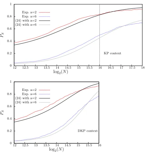
was on 6 rounds meaning that 2 rounds were partially inverted. In Figure 9, we give the results of the experiments.
0 0.2 0.4 0.6 0.8 1
12 12.5 13 13.5 14 14.5 15 15.5 16 16.5 17 17.5 18
PS
log2(N)
KP context Exp. a=2
Exp. a=6 (24) with a=2 (24) with a=6
0 0.2 0.4 0.6 0.8 1
12 12.5 13 13.5 14 14.5 15 15.5 16
PS
log2(N)
DKP context Exp. a=2
Exp. a=6 (24) with a=2 (24) with a=6
Fig. 9: Success probability of a key-recovery attack. The theoretical success probability is computed from Equation (24) using the normal distribution . The experimental results (Exp.) are represented with dotted lines. The parameters aren= 16,`= 26−1,
CR= 2−9.20,CW = 2−10. Top: Using non-distinct plaintexts (B= 1). Bottom: Using distinct plaintexts (B= 1−N/216).
6
Zero-Correlation Linear Cryptanalysis
6.1 Multiple and Multidimensional Zero-Correlation Linear Attacks
Zero-correlation linear cryptanalysis is a special case of multiple/multidimensional linear cryptanalysis withCR= 0 andCW =`2−n. Applying Corollary 2 we
ob-tain the following estimate of the data complexity of a multiple/multidimensional zero-correlation linear attack.
Corollary 3. The number NKP of known plaintexts required in a multiple or multidimensional zero-correlation linear attack is:
NKP ≈2
n(ϕ
P S+ϕa)
p
`/2−ϕa
. (26)
The numberNDKP of distinct-known plaintexts required in a multiple or
multi-dimensional zero-correlation linear attack is:
NDKP≈ 2
n(ϕ
P S+ϕa)
p
`/2 +ϕP S
Proof. The result is straightforward while puttingλ= 0 in Equation (25). ut
In [9, 11, 13], Equations (26) and (27) were given for respectively KP mul-tiple zero-correlation attacks and DKP multidimensional zero-correlation linear attacks. The results of this paper allows now to consider the two other cases: DKP multiple zero-correlation attacks and KP multidimensional zero-correlation attacks is backed up by experiments in the next section.
Since for most attacks 0.5 ≤PS ≤0.99, meaning that 0 ≤ϕPS ≤2.4, the difference between Equation (27) and Equation (26) is particularly noticeable when p`/2 and ϕa are in the same order of magnitude. From Equation (27)
and Equation (26) we deduce that the success probability of a known-plaintext zero-correlation linear attack is:
PS ≈Φ NKP
2n p
`/2−ϕa
NKP+ 2n
2n
, (28)
and the one of a distinct-known-plaintext zero-correlation linear attack is:
PS ≈Φ
NDKPp
`/2 2n−NDKP −ϕa
2n
2n−NDKP
!
. (29)
6.2 Experimental Results
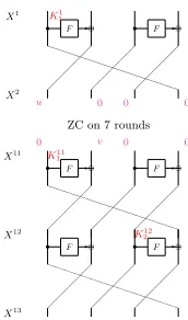
We have implemented experiments on a Feistel-type cipher which is depicted in Figure 10 and could correspond to scaled versions of CLEFIA [31] (a 16-bit type-II GFN with 4 branches) .
F F
s -e s -e
PPPPPPPPPPPPPPP
F F
s -e s -e
PPPPPPPPPPPPPPP
F F
s -e s -e
PPPPPPPPPPPPPPP
u 0 0 0
0 v 0 0
K1 1
K11 1
K12 2 X1
X2
X11
X12
X13
ZC on 7 rounds
Fig. 10: Description of the key-recovery attack done on a Type-II GFN.
While in [32] experiments showing the distribution of ExpD,K(T(D, KR)) and
ExpD,KW(T(D, KW)) have been presented, there is, to the best of our knowledge,
The results of our experimental attacks averaged over 1000 keys are provided in Figure 11. In these graphics we compare the success probability of multidi-mensional and multiple zero-correlation linear attacks with the theoretical ones given for KP by Equation (28) and for DKP by Equation (29). These experi-ments support the theory given in Section 6.1 showing that the same formula can be used to compute the complexity of multiple zero-correlation and multi-dimensional zero-correlation linear attacks. The difference lies only in the way of sampling, whether distinct or non-distinct known plaintexts are used in the attack. The bottom left graphic of Figure 11 corresponds to a case where only 32 approximations are taken into consideration. The gap between the theoret-ical and experimental success probability observed in these experiments is due to the approximation of the gamma distributions by normal distributions which is not accurate since` = 32. Using Equation 4 with the corresponding gamma distribution we obtain a more accurate estimate of the success probability of the attack.
0 0.2 0.4 0.6 0.8 1
10 11 12 13 14 15 16
PS
log2(N)
distinct non-distinct (29) (28)
0 0.2 0.4 0.6 0.8 1
10 11 12 13 14 15 16
PS
log2(N)
distinct non-distinct (29) (28)
Multidimensional`= 255,a= 4 Multidimensional`= 255,a= 11
0 0.2 0.4 0.6 0.8 1
12 12.5 13 13.5 14 14.5 15 15.5 16 PS
log2(N)
distinct non-distinct (29) (28)
0 0.2 0.4 0.6 0.8 1
12 12.5 13 13.5 14 14.5 15 15.5 16 PS
log2(N)
distinct non-distinct (29) (28)
Multiple`= 32,a= 6 Multiple`= 64,a= 6
6.3 Applications
Multiple zero-correlation linear attacks. As explained in detail later in this paper, by considering distinct-known plaintexts we can use Equation (27) to compute the data complexity of a multiple zero-correlation linear attack. As the data com-plexity of multidimensional linear attacks has already been computed under this setting, and because other comparable (in number of attacked rounds) attacks have been performed in the chosen-plaintext model, this should give us a better comparison factor. The result of our computation and a comparison with the best attacks on the block cipher Camellia [2] are provided in Table 1. The attack is from [9]. The data complexity has been computed using Equation (27) instead of using Equation (26) with the parameters of the attack chosen as PS = 0.85
anda= 96 ora= 160. The time complexity has been computed according to the description given in [9]. We use the abbreviations KP, DKP and CP for known plaintext, distinct-known plaintext and chosen plaintext, respectively.
Version #R Type ` a PS N Time Mem. Ref.
128 11 ID - - - 2118.4 CP 2118.43296.4 [14] 128 11 ZC 214 96 85% 2125.3 KP 2125.8 2112 [9] 128 11 ZC 214 96 85%2125.1 DKP 2125.8 2112 Equation (27)
192 12 ID - - - 2119.7 CP 2161.062147.7 [14] 192 12 ZC 214160 85% 2125.7 KP 2125.8 2112 [9] 192 12 ZC 214160 85%2125.46 DKP2125.8 2112 Equation (27) Table 1: Best key-recovery attacks on Camellia-128 and Camellia-192 (attacks start-ing from the first round). The memory is expressed in number of bytes. #R denotes the number of attacked rounds. ID stands for impossible differential, ZC for zero-correlation.
Similarly we can improve the data complexity of the multiple zero-correlation linear attack on CAST-128 [34]. The parameters of the attack being n = 128, `= 64770,a= 50 andPS = 0.85, the data complexity of the attack using known
plaintextsfootnoteWith these parameters, the data complexity can not be equal to 2123.2 as given in [34]. is N = 2123.73 and the data complexity of the attack using distinct-known plaintexts isN= 2123.67.
Key-difference-invariant-bias attacks. Key-difference-invariant-bias attack is a
![Fig. 4: The round function of SMALLPRESENT-[8] (left) and SMALLPRESENT-[4](right).](https://thumb-us.123doks.com/thumbv2/123dok_us/7924561.1315801/23.612.163.465.460.599/fig-round-function-smallpresent-left-smallpresent-right.webp)
![Fig. 5: The mean ExpD,K(T(D, KR)) for a 6-bit multidimensional distribution (ℓ =26 − 1) over 4 rounds of SMALLPRESENT-[4] with capacity C = 2−9.20.](https://thumb-us.123doks.com/thumbv2/123dok_us/7924561.1315801/24.612.200.408.353.497/fig-mean-expd-multidimensional-distribution-rounds-smallpresent-capacity.webp)
![Fig. 6: The mean ExpD,K(T(D, KR)) for a 8-bit multidimensional distribution (ℓ =28 − 1) over 9 rounds of SMALLPRESENT-[8] with capacity C = 2−21.29.](https://thumb-us.123doks.com/thumbv2/123dok_us/7924561.1315801/25.612.200.409.123.266/fig-mean-expd-multidimensional-distribution-rounds-smallpresent-capacity.webp)
![Fig. 7: The variance VarD,K(T(D, KR)) for a 6-bit multidimensional distribution (ℓ =26 − 1) over 4 rounds of SMALLPRESENT-[4] with capacity C = 2−9.20.](https://thumb-us.123doks.com/thumbv2/123dok_us/7924561.1315801/26.612.200.408.118.265/fig-variance-vard-multidimensional-distribution-rounds-smallpresent-capacity.webp)
![Fig. 8: The variance VarD,K(T(D, KR)) for a 8-bit multidimensional distribution (ℓ =28 − 1) over 9 rounds of SMALLPRESENT-[8] with capacity C = 2−21.29.](https://thumb-us.123doks.com/thumbv2/123dok_us/7924561.1315801/27.612.199.409.121.265/fig-variance-vard-multidimensional-distribution-rounds-smallpresent-capacity.webp)