Collaborative Filtering Recommendation Algorithm Using Implicit Similarity In Preference Relationships

Collaborative Filtering Recommendation Algorithm Using

Implicit Similarity in Preference Relationships

Yu Hong ZhouP

[*]

P

, Zhi Jie Duan, Wei Jiang

*Chongqing Key Lab of Mobile Communications Technology, Chongqing University of Posts and Telecommunications, Chongqing 400065, P. R. China

Abstract

In traditional collaborative filtering recommendation algorithm, the similarity is calculated based on the common ratings and the accuracy is not well when the data is sparse. The thesis proposes a novel collaborative filtering by using implicit similarity in preference relationships(CF-ISP). Firstly, it divides the user group based on the user attributes, and secondly, it defines the item preference in the user group and calculates the preference similarity between the items. Finally, it introduces the preference similarity to the Probabilistic Matrix Factorization recommendation algorithm.The thesis conducts the experiment to verify the validity and the accuracy of the algorithm.

Keywords: Recommendation System, Collaborative Filtering, preference similarity,user group

1.

Introduction

With the explosive growth of the personalized recommendation technologies, the users can get higher quality service and better user experience, the items on the website can be displayed in front of the users who are really interested in them. Recommender systems enhances the economic efficiency of the website and the retention rate of the users on the platform[1]. For some time, the collaborative filtering technology is widely used in the industry because of it’s low dependence, good applicability and simple encoding. But it also faces the great challenges such as data sparsity problem. There are at least millions of users and items in the large business recommender systems, but the user only rate some of these items and caused data sparsity problem. Moreover, personalized recommendation also faces cold start problem, extendibility problem and so on.

For the sake of those problems, we first divide the user group based on the user attributes, and then calculates the

preference similarity between the items. Finally, it introduces the preference similarity to the Probabilistic Matrix Factorization recommendation algorithm. It first uses the user’s age attribute, gender attribute and preference attribute to calculate the interest distance between the different users, and utilizes the k-medoids method to divide the user group, and then the formal definition of the item preference is given to calculate preference similarity. Finally, it introduces the preference similarity to the Probabilistic Matrix Factorization recommendation algorithm and redefine the item’s potential feature vector. The local optimum of the potential feature vector can be obtained according to the matrix factorization and SGD method. The experimental result shows that the proposed algorithm utilizes the additional item’s information efficiently, enriches data source and improves the precision of the similarity computation, meets the personalized recommendation demands.

between the users that can spread just like the trust in social network, it constructs new user relationships to alleviate the data sparsity by spreading the similarity in bipartite graphs. Work in [7] proposes the textonly-based, hashtag-based and URL-based approaches to model user profiles and calculated the relevance between users. Work in [8] proposed a matrix factorization method to estimates unknown user-to-user rating based on given trust relation and rating records between social network users. Work in [9] considers that the tag reflects the semantic of the item rather the user’s preference, it recommends according to the different role of the tags to build the user-centric tripartite graph and the item-centric tripartite graph.

2.

User group division

2.1 related definition

Define user set U=

{

u u1, 2,...,um|m=|U|

}

, given a

positive integer K and division method, if Uis divided

non-empty subset

U

_lof size k, and

1

K

l l

U

U

=

=

∑

, we say

l

U

is one user group.

Define

a u

′

( )

and

g u

′

( )

represents the user age attribute

value and gender attribute value, the calculation as follows:

( ) ( ) min( ) max( ) min( )

i

a u a

a u

a a

− ′ =

− (1)

0 ( ) male

( )=

1 ( )=female

g u g u

g u =

′



_



，

， (2)

Define

d u v

( , )

represents the interest distance between the user u and the user v , the calculation as follows:

( , )

age

( , )

gender

( , )

pref

( , )

d u v

= ⋅

α

d

u v

+ ⋅

β

d

u v

+ ⋅

γ

d

u v

(3

)

Where

d

_age

( , )

u v

represents the age attribute distance,

( , )

gender

d

u v

represents the gender attribute distance,

( , )

pref

d

u v

represents the preference attribute distance, parameter α ,

β

and

γ

is weight factor and

1

α β γ

+ + = .

d

_age

( , )

u v

,

d

_gender

( , )

u v

and

d

_pref

( , )

u v

calculates as follows:

( , ) |

( )

( ) |

age

d

u v

=

a u

′

−

a v

′

(4)

( , ) |

( )

( ) |

gender

d

u v

=

g u

′

−

g v

′

(5)

( ( ( ), ( )))

( , )

( )

pref

h

H T p u p v

d

u v

H T

=

(6)

Where T p u( ( ), ( ))p v is a subtree, and the node

p u

( )

and

node

p v

( )

minimum common parent node as the subtree

root node,

T

_h is preference classification tree, H T( ) represents the height of the tree.

Define bipartite graph model G < U, E, w >, U is the user

node set, E is the edge set,

e v v

( , )

_{u i}

∈

E

represents there is an edge connect the node

v

_u and

v

_i , the weight

( , )

_{u i}

w v v

represents the interest distance of the user node

u

v

and

v

_i. The user interest distance matrix M as follows:

[

( , )]

_{m m}

M

=

dist i j

×

(7)

Where

dist i j

( , )

is the interest distance between the user

i

and user

j

.

2.2 user group division

The pseudocode of the collaborative filtering recommendation algorithm using implicit similarity in preference relationships as follows:

CF-ISP algorithm pseudocode

Algorithm: Collaborative Filtering Recommendation Algorithm Using Implicit Similarity in Preference Relationships

Input: user interest distance matrixMR

, Rthenumber of user group N, user u

Output: N user groups

1: initialize

{

}

1

,

2

...

N

G

=

g g

g

2: initialize

{

}

1

,

2

,...,

c k

C

=

c c

c

3: while

||

M

_{in dist_}

[

c

_kt+1

][

c

_kt

||

₂2

<

ε

do 4: for each user u_i∈U do

5: for each medoid c_i∈C_c do 6:

dis u c

( , )

_{i i}

=

M

_{in dist_}

[ ][ ]

u

_i

c

_i 7: end for

8:

_{( ,}

₎

_min

{

_{[ ][ ],...,}

_{[ ][ ]}

}

i m i m i k

dis u c

=

M u c

M u c

9:

g

_m

=

c

_m



u

_i

10: end for

11: for each user

u

_i

∈

g

_i

& &

u

_i

≠

c

_i do 12: for each user

u

_j

∈

g

_i

& &

u

_j

≠

c

_i 13:

dis

_

sum u

( )

i

+ =

M

in dist_{_}

[ ][

u

i

u

j

]

14: end for

15:

u

_i

=

min{

dis

_

sum u

( ),...,

₁

dis

_

sum u

(

_m

)}

16: end for

17:

c

_i

=

u

_i 18:return

3.

Implicit similarity in preference

In the previous section, we divide the user to k user groups. For each user group, we divide the original rating

matrix into R=R₁R₂ ... R_k , the submatrix

R

_i is consist of all users and rating item and rating point in

i

-th

user group.

Define user set

U

=

{

u u

₁

,

₂

,...,

u

_m

}

, any item

i,

{

,

}

( ) | _{u i}

U i = u∈U R ≠ ∅ represents the user set who has

rated the item

i,

∀ ∈

C

_k

C

| ( ) |

( ) (0 ( ) 1)

| ( ) |

k

C U i

pref i pref i

U i α

= ≤ ≤

+



(8)

( )

pref i represents the item’s preference in the user group

k. We construct the item-user group preference matrix by the preference value, as table 1 shows:

item-user group preference matrix

1

c

…

c

j

…

k

c

1

item

P

1,1

…

1,j

P

…

P

_1,k

… … … … … …

j

item

P

_j,1 …

P

_{j j,} …

P

_{j k,}

… … … … … …

n

item

P

n,1

…

,

n j

P

…

P

_{n k,} Where

P

_{n k,} represents the preference of the item

item

_n in user group

c

_k.

Define item set

{

}

1, , ...,2 k

I = i i i

, and

∀ ∈

i

I

, it

uses

(

)

,1

,

,2

,...,

, i i i k

P P

P

=

i

f

represents the preference

feature vector of the item i, and the implicit similarity in

preference relationships between the item

i

and item

j

can represent as follows:

1

2 2

1 1

( , ) cos( , )

k in jn n

k k

in jn

n n

p p sim i j

p p

=

= =

= =

∑

∑

∑

i j

f f (9)

4.

Recommendation algorithm CF-ISP

Fig 1:CF-ISP model

The thesis redefines the item’s potential feature vector as follows: _, j

ˆ

V =

i

i j i j N

V S

∈

∑

(10)

Where

N

_i

is

the neighbor set of the item

i

,

S

_{i j,} is implicit similarity in preference relationships between item

i

and item

j

, and _,

( )

1

i j j N i

S

∈

=

∑

. The Conditional

Distributions of the rating matrix Rdefine as follows:

2 2 , 1 1

( |

, ,

)

[ (

| (

),

)]

R ij m n I T

R i j i j R

i j

p R U V

σ

N R

g U V

σ

= =

=

∏∏

(11)

Where I_ijR is the feature function, if the user U_i has rated

the item V_j I_ijR =1else I_ijR =0.

Based on the Bayes theorem and likelihood function of Eq.(11) we can obtain the posterior probability of U and

V :

2 2 2 2

2 2 2 2

( , | , , , , , )

( | , , ) ( | ( | ,

R S U V

R U V S

p U V R S

p R U V p U p V S

σ σ σ σ

σ σ σ σ

∝ ） , ）

(12)

Where

p V S

( | ,

σ σ

V2

,

S2

）

∝

p V S

( | ,

σ

S2

)

×

p V

( |

σ

V2

)

the thesis incorporates the implicit similarity sim i j( , ) into

PMF, so p V S( | ,σ_S2) can be defined as follows:

2 2 , 1

( | ,

)

(

|

,

)

i N

S i j i j S

j N i

p V S

σ

N V

V S

σ

I

∈ =

=

∏

∑

(13)

We proposed by minimizing its arithmetic negation

function L R U V S_F( , , , ) , the task is transformed to the

following minimization problem:

(

)

, ,

1 ( ) ( )

1 1 2 , , 1 1

( , , , )

2

+ (14)

2

2

T N

S

F i j i j i j i j

i j N i j N i

M N

T T

U V

u u i i

u i

M N

R T

u i u i u i u i

L R U V S

V

V S

V

V S

U U

V V

I

R

U V

λ

λ

λ

= ∈ ∈ = = = =

=

−

−

+

+

−



_

_{ }

_





_

_{ }

_





_

_{ }

_







∑

∑

∑

∑

∑

∑∑

Where

λ

U

=

σ σ λ

R2 U2

,

V

=

σ σ λ σ σ

R2 V2

,

s

=

R2 S2 are

the regularization to avoid model overfitting. To minimize

the objective function L R U V S_F( , , , )in Eq.(14), we use

the gradient descent on ∂L_F ∂U_u and ∂L_F ∂V_i for each

pair U_u and V_i, as follows:

, , 1

(

)

N R T F

u i i u i u i U u i

u

L

I V U V

R

U

U

=

λ

∂

=

−

+

∂

∑

(15)

, , 1 , ( ) , | ( ) ( )

(

)

(

)

(

)

M R T F

u i u u i u i i

i

V i S i j i j j N i

S j x j x

j i N j x N j

L

I U U V

R

V

V

V

V S

V

V S

λ

λ

λ

= ∈ ∈ ∈

∂

=

−

+

∂

+

−

−

−

∑

∑

∑

∑

(16)

5.

Experiment

5.1 Datasets

In our experiments, we used the MovieLens10M datasets, it contains 71567 users, 10681 movies. We evaluated the completion by RMSE(Root Mean Square Error) 1 j V u U , u i R

..

.

i V 1 , i j S 2 , i j S 2 j V w j V ,w i j S V σ U σ S σ 1, 2,...,

i= N

1, 2,...,

u= M

2 R

3.2 experiment result

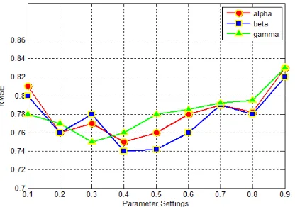
Fig.2: parameter and RMSE corresponding relation

In Figure 2, the experimental results are

presented. When

α

=0.4β =0.4 ~ 0.5γ =0.3

,

the

RMSE attain optimal value changes with the parameter. When β =0.4 ~ 0.5 , RMSE reaches

minimum 0.74. So we consider the user attribute that the parameter

β

corresponds to has the most influential and importance to the recommender results. It reintroduces the condition

α β γ

+ + =1we can draw

a conclusion that when

0.4

β

=

,

_α

_=0.35

,

_γ

_=0.25

,

RMSE reaches minimum and achieve best performance of recommendation.

Fig.3: k and RMSE corresponding relation

In Figure 3, the experimental results are presented. The RMSE decreases with increasing of user group k, when

_k

=

₅₀

RMSE reaches minimum 0.74. Continue increasing k, RMSE increases and it reduces the recommendation quality.

Table 1 :

λ

_S and RMSE corresponding relation

S

λ

f

=

5

f

=

10

0.001 0.7655 0.7632

0.01 0.7476 0.7459

0.1 0.7459 0.7433

0.5 0.7572 0.7569

1 0.7667 0.7661

5 0.7702 0.7698

10 0.7798

0.7729

In Table 1, it is easy to find that in the same

dimension, changes in parameter

λ

_S has the great influential to RMSE. RMSE decreases with increasing of

S

λ

, when

λ

_S∈[0.01, 0.1], RMSE descends to its lowest level.

Fig.4: feature number and RMSE corresponding relation

In Figure 4, the experimental results are presented. RMSE decreases with increasing of feature number f , when f =10 RMSE descends to its lowest level.

Increasing

f

, the performance of the recommender system starts to slide, But the CF-ISP algorithm still has the lowest RMSE compared to the other three algorithms.

6.

Conclusions

In this thesis, we have proposed a new collaborative filtering recommendation algorithm CF-ISP which leverages preference information to improve the recommendation result. The thesis first divide the user group based on the user attributes, and then calculates the

10 20 30 40 50 60 70 80 90 0.72

0.73 0.74 0.75 0.76 0.77 0.78 0.79 0.8

number of user groups(k)

RM

S

E

0.5 0.6 0.7 0.8 0.9 1

RM

S

E

Item-MEAN PMF CTR CF-ISP

preference similarity between the items. Finally, it introduces the preference similarity to the Probabilistic Matrix Factorization recommendation algorithm. The experiment result shows that CF-ISP excels other peer algorithms in terms of recommendation evaluation metrics. As the future work, we plan to parallelize the algorithm, and increase the amount of experimental data.

References

[1] Groh G, Ehmig C. Recommendations in taste related domains: collaborative filtering vs. social filtering[C]//Proceedings of the 2007 international ACM conference on Supporting group work. Sanibel: ACM Press, 2007: 127-136.

[2] Ma H, King I, Lyu M R. Effective missing data prediction for collaborative filtering[C]// SIGIR 2007: Proceedings of the, International ACM SIGIR Conference on Research and Development in Information Retrieval, Amsterdam, the Netherlands, July. DBLP, 2007:39-46. [3] V. Agarwal and K. K. Bharadwaj. A collaborative filtering framework for friends recommendation in social networks based on interaction intensity and adaptive user similarity.Social Network Analysis & Mining, 3(3):359-379, 2013.

[3] Wang S, Xie Y, Fang M. A collaborative filtering recommendation

algorithm based on item and cloud model[J]. Wuhan university journal of

natural sciences, 2011, 16(1): 16-20.

[4] Ahn H J. A new similarity measure for collaborative filtering to alleviate the new user cold-starting problem[J]. Information Sciences, 2008, 178(1):37-51.

[5] Y. Koren. Factor in the neighbors: Scalable and accurate collaborative filtering. ACM Transactions on Knowledge Discovery from Data (TKDD), 4(1):1–24,Jan. 2010.

[6] Satsiou A, Tassiulas L. Propagating Users' Similarity towards Improving Recommender Systems[C]// Web Intelligence. ACM, 2014:221-228.

[7] M. Chechev and P. Georgiev. A multi-view content-based user recommendation scheme for following users in twitter.In Social Informatics, pages 434-447. ACM, 2012.

[8] Jamali, M. and Ester, M. 2010. A matrix factorization technique with trust propagation for recommendation in social networks. In Proceedings of the fourth ACM Conference on Recommender Systems(Sept 26-30, 2010,Barcelona, Spain), RecSys’2010, ACM, 135-142.DOI=http://doi.acm.org/10.1145/1864708.1864736.

[9] Firan C S, Nejdl W, Paiu R. The benefit of using tag-based profiles[C]//Web Conference, 2007. LA-WEB 2007. Latin American. IEEE Press, 2007: 32-41.

YuHong Zhou, was born in Tongling of Anhui province in 1989.

He is now a graduate student in Chongqing University of Posts

and Telecommunications. Hisresearch concerns Mobile communication techniques..

Zhi Jie Duan, was born in Jian of JiangXi province in 1992. He is

now a graduate student in Chongqing University of Posts and Telecommunications. His research concerns Mobile communication techniques.

Wei Jiang was born in ZheJiang province in 1992. He is now a