1845
CLASSIFICATION OF PNEUMONIA PATIENTS RISK USING
HYBRID GENETIC ALGORITHM-DISCRIMINANT
ANALYSIS AND NAÏVE BAYES
1IRHAMAH, 2SITI MAR’ATUS RAHIMATIN, 3HERI KUSWANTO, 4LAKSMI WULANDARI
1,2,3Department of Statistics, Institut Teknologi Sepuluh Nopember, Surabaya, Indonesia
4Faculty of Medicine, Universitas Airlangga, Surabaya, Indonesia
E-mail: 1[email protected]
ABSTRACT
Pneumonia is the most common causes of death in developing countries, such as in Indonesia. Therefore, appropriate pneumonia classification is very important in determining the disease severity and to know the most appropriate treatment for the patient. In this study, Discriminant Analysis (DA), hybrid Genetic Algorithm- Discriminant Analysis (HGA-DA) and Naïve Bayes (NB) are used to classify risk class of patient. GA is an artificial intelligent method that can avoid a trap in local optima and easy to implement in solving various objective functions and constraints, while NB is a simple but powerful method that returns not only prediction but also the degree of certainty. In this study, GA is used to improve multi-class classification performance of DA. Firstly, GA is used for variable selection in DA, and then a comparative study with other variable selection methods is performed. In addition, Genetic Algorithm is also implemented for parameter estimation. Analysis results show that there are differences in selected variables from four selection methods in classifying patient risk class. The use of hybrid methods of DA and GA in variable selection and parameter optimization stages gives better multi-class classification results than DA or NB, since it produces highest Geometric Mean (GM) and Area Under Curve (AUC) criterion.
Keywords: Pneumonia, Multi-class Classification, Discriminant Analysis, Genetic Algorithm, Naïve Bayes
1. INTRODUCTION
Pneumonia is a type of disease that causes serious problems that can lead to consolidation of lung tissue and disturbances of local gas exchange, and also cause high morbidity [1]. According to the Basic Health Research (RISKESDAS) [2], the prevalence of pneumonia in Indonesia in 2013 is 4.5%. Compared to other provinces in Java, East Java has the highest prevalence of Acute Respiratory Infection (ARI) that is 4.2%. Pneumonia is typically grouped into community acquired (Community Acquired Pneumonia) and hospital admissions (Hospital Acquired Pneumonia) [3]. Community pneumonia (CAP) is ranked on fourth of the ten most-treated diseases per year [4].
Early examination is necessary in the prevention of pneumonia. Knowing the level of classification of the disease is very important in order to accelerate the determination of the most appropriate treatment for the patient. Assessment
on the severity of pneumonia is an important component in the management of community pneumonia. This led to the emergence of various scoring systems such as PSI, CURB-65, modified ATS (m-ATS) and so forth [3]. Some commonly used scoring systems are the PSI system (Pneumonia Severity Index) developed by the PORT (Pneumonia Patient Outcome Research Team) recommended by the American Thoracic Society Guidelines (ATS) and the CURB-65 system which is a recommendation from the BTS (British Thoracic Society).
1846 selection and parameter estimation of discriminant function in classifying pneumonia patients’ risk class. Furthermore, the results will be compared to Naïve Bayes classification method result. Although included in a simple classification method, a study conducted by [7] concludes that Naïve Bayes produced a higher classification accuracy than the Artificial Neural Network method. Another study conducted by [8] gives the conclusion that the Naïve Bayes method has the highest accuracy value compared to the Support Vector Machine (SVM) and Random Forest methods. Hence, in this research, a comparative study of the performance of Discriminat Analysis, Hybrid Genetic Algorithm- Discriminat Analysis and Naïve Bayes to classify pneumonia patients risk are conducted.
2. DISCRIMINANT ANALYSIS
Discriminant Analysis is a multivariate technique concerned with separating distinct sets of objects and to allocate new objects into previously defined groups. Discriminant analysis is one of the dependency techniques, finding the effect of the dependent variable based on several independentvariables [9]. Discriminant analysis works when the measurements made on categorical dependent variable and continuous independent variables [10]. Discriminant analysis is one of statistical methods that can be used for classification. The linear discriminant function takes form of a linear combination of coefficients of p variables and their respective variables in the study as equation(1).
A variate of the independent variables selected for their discriminatory power used in the prediction of group membership. The predicted value of the discriminant is the discriminant Z score, which is calculated for each object in the analysis. It takes the form of the linear equation (1).
1 1 2 2
...
ji i i p pi
Z
a w x
w x
w x
(1)
where
𝑍 : discriminant Z score of discriminant function j
for object i
𝑎 : constant/ intercept
𝑤 : discriminant weight for the independent variable p
𝑥 : independent variable p and object i [10]
In discriminant analysis, there are assumptions that must be fulfilled prior to performing the analysis:
(1) The data follows a multivariate normal distribution
The Mardia test can be used to test the null hypothesis H0 of multivariate normality. The Mardia’s skewness statistic for this hypothesis is
MS 𝑛
6𝛾, (2)
and Mardia’s kurtosis statistic
MK 𝛾 , (3)
where
𝛾,
1
𝑛 𝑚 (4)
𝛾, 𝑛1 𝑚 (5)
with 𝑚 𝑥 𝑥̅ 𝑥 𝑥̅ is mahalanobis distance. [11]
(2) Homogeneity of variance-covariance matrices. Box's M tests the null hypothesis of homogeneity of covariance matrices.
(3) Equality of Group Means
The tests of equality of group means measure each independent variable's potential before the model is created
Variable selection methods used in this study are stepwise method, forward selection, backward elimination and genetic algorithm. The details of the method are given as follows:
1. Stepwise Method
It involves entering the independent variables into the discriminant function one at a time on the basis of their discriminating power. The stepwise approach follows sequential process of adding or deleting variables in the following manner:
- Choose the single best discriminating variable
- Pair the initial variable that is best able to improve the discriminating power of the function in combination with the first variable.
1847 previously selected variables may be removed if the information they contain about group differences is available in some combination of the other variables included at later stages.
- Consider the process completed when either all independent variables are included in the function or the excluded variables are judged as not contributing significantly to further discrimination. [10]
2. Backward Elimination
Discriminant analysis is performed by using model containing all independent variables. Then the independent variable having the smallest partial F value or largest Wilks’ Ʌ value is chosen. If 𝑝 indicates that this independent variable is significant at the 𝛼level then the procedure terminates by choosing the model containing all independent variables. If this independent variable is not significant at the 𝛼 level or 𝑝 𝛼, it is removed from the model and the discriminant analysis is performed by using all the remaining independent variables. At each step an independent variable is removed from the model if it has the smallest partial F value and it is not significant at the 𝛼 level. The procedure terminates when no independent variable in the model can be removed.
3. Forward Selection
Variable selection is done by entering one by one independent variable that has the largest partial F value and 𝑝 𝛼.
4. Genetic Algorithm
This method selects the predictor by selecting combination of variables that produces the best fitness value.
The coefficients are estimated such that the function maximizes the distance between the two centroids. That happens when a ratio (λ)-between group sum of squares to within group sum of squares is maximized [12]. Then the vector of coefficients a that maximizes the ratio given as follows.
𝛂 𝑩𝛂 𝛂 𝑾𝛂
𝛂 ∑ 𝒙⃗ ̅ 𝒙 𝒙 𝛂
𝛂 ∑ ∑ 𝒙 ̅ 𝒙 𝒙 𝛂
(6)
where:
𝛂 =coefficient vector of discriminant function
𝒙 = mean vector
𝒙 = measurement on independent variable j and category k
Then we calculate the value of discriminant function for the classification and then allocate x to
l
if2 2 2
1 1 1
ˆ ˆ ˆ
( ) [ '( )] [ '( )] ,
r r r
j lj j l j m
j j j
y y a x x a x x l m
(7) where 𝑎′ is parameter coefficient vector,
ˆ '
lj j l
y
a x
and𝑟 𝑠. x will be allocated to 𝜋when the value of ∑ 𝑦 𝑦 is minimum. The performance of classification function can be evaluated by calculating the geometric mean (GM) and Area Under Curve (AUC) using formula below.
𝐺_𝑚𝑒𝑎𝑛 𝑅 (8)
𝐴𝑈𝐶 1
𝑘 𝑅 (9)
Where
𝑅 𝑛
∑ 𝑛 , 𝑗 1,2, . . , 𝑘 (10)
3. GENETIC ALGORITHM
The Genetic Algorithm is used to solve both constrained and unconstrained optimization problems based on natural selection, the process that drives biological evolution. Genetic algorithm can used to solve a variety of optimization problems that are not well suited for standard optimization algorithms, including problems in which the objective function is discontinuous, non-differentiable, stochastic, or highly non-linear [13]. Each iteration consists of the following steps [14]: (i) Initialization: The initialization value used
comes from the encoding of a gene in chromosome which represents the individual genes.
(ii) Evaluate the fitness of each chromosome in the population.
(iii) Selection: Apply Roulette Wheel Selection where each chromosome occupies a circular piece of roulette wheel proportionately according to the fitness value.
1848 (v) Mutation: used to prevent the algorithm from
being trapped in the optimum local solution [15].
(vi) Evaluation. Then the fitness of the new chromosomes is evaluated.
(vii) Replacement. During the last step, individuals from the old population are replaced by the new ones.
(viii) Elitism. Save and copy several best chromosomes into next iteration.
4. NAÏVE BAYES CLASSIFIER
Naive Bayes is one of the simplest probabilistic classifiers based on the Bayes theorem. Naïve Bayes Classification is statistical classification method can be used for predicting membership of class [16]. Generally, Bayes theorem can be formulated as
𝑃 𝐴|𝐵 𝑃 𝐴 𝑃 𝐵|𝐴
𝑃 𝐵 (11)
If there is a quantitative or continuous attribute, then 𝑃 𝑋 |𝑌 will be calculated using normal distribution approach
𝑃 𝑋 |𝑌 1
𝜎 √2𝜋𝑒𝑥𝑝
𝑋 𝜇
2𝜎 (12)
Probability estimation 𝑃 𝑋 |𝑌 can be calculated for each attribute 𝑋 and class Y so that new data can be classified into certain Y based on largest probability value among it.
5. PNEUMONIA
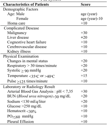
[image:4.612.317.528.111.358.2]Pneumonia is an inflammation that affects the lung parenchyma that leads to consolidation of lung tissue and local gas exchange disturbances [17]. The first management of pneumonia patients after being diagnosed is the determination of the treatment site based on the severity of pneumonia. Assessment of the severity of pneumonia is an important component in the management of community pneumonia. Some of the commonly used scoring systems are the PSI system (Pneumonia Severity Index) developed by the American Thoracic Society Guidelines (ATS) and the CURB-65 system which is a recommendation from the BTS (British Thoracic Society) [3]. These scores are also used as a guide for selection of antibiotic therapy and morning treatment of patients with pneumonia. PSI Scoring System is presented in Table 1 and 2.
Table 1: Scoring System on Community Pneumonia PSI System
Characteristics of Patients Score Demographic Factors
Age: Male age (year) Female age (year)-10
Homa care +10
Complicated Desease
Malignancy +30
Liver disease +20 Cognestive heart failure +10 Cerebrovascular disease +10 Kidney illness +10 Physical Examination
Changes in mental status +20 Respiratory > 30 times/minute +20 Systolic ≥ 90 mmHg +20 Temperature <35ᵒC or >40ᵒC +15 Pulse ≥125 times/minute +10 Laboratory or Radiology Result
Arterial Blood Gas Analysis : pH < 7,35 +30 BUN (Blood urea nitrogen)>30 mg/dL +20 Sodium <130 mEq/liter +20 Glucose >250 mg/dL +10 Hematocrit <30% +10 PO2≤60 mmHg +10
Pleural Effusion +10
[image:4.612.311.526.447.520.2]Then the points of the PORT result are summed up. The summations are then categorized according to the risk class, so that appropriate treatment can be determined.
Table 2: Risk Score with PSI System
Risk Class Total Score
Recommendation
Low I 0 Outpatient II <70 Outpatient III 71-90 Inpatient/Outpatient Intermediate IV 91-130 Inpatient
High V >130 Inpatient
In addition, the CURB-65 system is a very practical, memorable and valuable score model. The advantages of this score are its easy use and are designed to better assess disease severity rather than assessing pneumonia patients with mortality risk. The CURB-65 system is given in Table 3.
Table 3: Prediction Score of CURB-65
Characteristics Score Loss of consciousness 1 Blood Urea Nitrogren> 20 mg/dL 1 Respiratory Frequency 30 per minute 1 Blood preassure (systolic < 90 mmHg or diastolic 60 mmHg)
1
1849 Then the CURB-65 score is summed and categorized based on its severity as shown in Table 4.
Table 4: Risk Classes with CURB-65 System
Total Score
Risk Classes Recommended Treatment 0 Low Outpatient 1 Low Outpatient
2 Intermediates Inpatient / Outpatient 3 Intermediates to High Inpatient / Outpatient 4 or 5 High Inpatient/ ICU
6. PROCEDURE
The data used in this research is a secondary data obtained from medical record data of pneumonia patients at hospital ‘T’ in Surabaya. The data consists of samples of pneumonia patients in 2015. The Pneumonia patient data is classified into 4 categories of dependent variables, 5 independent variables and 196 observations. The variables used in this study are shown in Table 5.
Table 5: Research Variables
Symbol Variable Scale
Y Risk Class: I/II/III/IV/V Ordinal
X1 Age (years) Rasio
X2 Systolic (mmHg) Rasio
X3 Diastolic (mmHg) Rasio
X4 Respiratory Frequency per minute Rasio
X5 Blood Urea Nitrogen (mg/dL) Rasio
The steps of the analysis are described below. 1. Perform descriptive statistics and data
exploration.
2. Partitioning data into training data and testing data with a ratio of 90:10 and 80:20
3. Selecting variables in discriminant analysis using forward selection, backward elimination, stepwise method, and genetic algorithm. The steps in variable selection using the genetic algorithm as follows:
a. Representing the independent variable into the chromosome and determines the initialization value.
b. Evaluating chromosomes based on fitness values, namely the value of misclassification.
c. Making a selection process with roulette wheel selection (RWS).
d. Crossovers with probability of crossing (Pc)
is 0.8
e. Perform mutation processes with mutation probabilities (Pm) is 0.1 and
f. Carry out the elitism process.
g. Change the old population with a new generation.
h. Repeating the process from step d until convergent fitness value is get
4. Perform discriminant analysis :
a. Test the assumption of multivariate normal distribution, the homogeneity of variance-covariance matrix and the groups mean difference for the entire independent variable.
b. Detect multicollinearity among independent variables.
c. Estimating the coefficients of the discriminant function parameters.
d. Calculate the GM and AUC from testing dataset
5. Estimate parameter using genetic algorithms with similar steps such as in variable selection, the difference is in the chromosome representation.
6. Analyzing data using Naїve Bayes
a. Calculate the probability value of each parameter in each category.
b. Determine the final probability of all parameters for each category.
c. Determine the category group based on the highest probability value.
d. Calculate the GM and AUC for testing dataset
e. Compare the value of classification performance criterions from the results of analysis using discriminant analysis methods, hybrid discriminant analysis-genetic algorithms and Naive Bayes. 7. Draw a conclusion
7. RESULTS AND DISCUSSION
7.1 Characteristics of Pneumonia Patients at Hospital ‘T’ in Surabaya
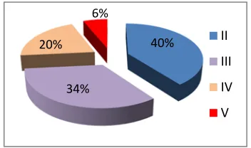
[image:5.612.330.506.599.703.2]Pneumonia patient's medical record data consist of 5 categories on dependent variable, but there is no patient included in class 1 category so the number of categories is 4 with total 96 observations. Based on Figure 1, it shows that the proportion of each category is imbalanced.
Figure 1: Proportion of Each Class of Pneumonia Risk
40%
34% 20%
6%
II
III
IV
1850 7.2 Discriminant Analysis Results
Before performing discriminant analysis, the data is firstly partitioned into training data and testing data with proportions of 90:10 and 80: 20. Furthermore, the discriminant analysis assumptions testing and multicollinearity detection are conducted. The results are as shown in Tabel 6.
Table 6: The Result of Discriminant Assumption Testing (90:10 split)
Assumption Test Statistics pvalue
Multivariate Normal
Mardia
Skweness 246.509 0.000
Mardia
Kurtosis 4.621 0.000
Homogeneity of Variance and Covariance Matrices
Box’s M 41.978 0.003
The table showed that both assumptions of normal multivariate distribution and homogeneity variance-covariance matrices are violated. To overcome this, the data need to be transformed using Box Cox transformation as in Table 7.
Table 7: Lambda Value of Box-Cox Transformation (90:10 split)
Variable Lambda value
𝑋 1.00
𝑋 -0.50
𝑋 0.50
𝑋 -0.50
𝑋 0.00
Furthermore, multivariate normality is tested for transformed data, and also the homogeneity variance-covariance assumption as shown in Table 8. After suitable transformation, both assumptions of normal multivariate distribution and homogeneity variance-covariance are satisfied.
Table 8: The Result of Assumption Testing of Transformed Data (90:10 split)
Assumption Test Statistics pvalue
Multivariate Normal
Mardia Skweness
46.959 0.085
Mardia Kurtosis
0.5809 0.561
Homogeneity of Variance and
Covariance Matrices Box’s M 60.319 0.176
Furthermore, the Equality of Group Means test is performed for each independent variable as summarized in Table 9
.
Table 9 shows that the hypothesis of equality of group means is rejected for 𝑋 and 𝑋 .Table 9: Equality of Group Means Test Result from Transformed Data (90:10 split)
Variable Wilks' Lambda pvalue
𝑋 0.623 0.000
𝑋 0.979 0.309
𝑋 0.982 0.380
𝑋 0.927 0.004
𝑋 0.736 0.000
Next, multicollinearity detection is performed.
Table 10: Correlation among independent variables (90:10 split)
𝑿𝟏 𝑿𝟐 𝑿𝟑 𝑿𝟒
𝑿𝟐 0.259 0.001*
𝑿𝟑 0.064 0.403* 0.710 0.000*
𝑿𝟒 -0.121 0.112* -0.161 0.033* -0.045 0.558*
𝑿𝟓 0.307 0.000* -0.049 0.524* -0.031 0.679* 0.079 0.300*
* 𝑝
Based on Table 10, it can be seen that the correlation among several independent variables are significant. A high correlation value indicates a case of multicollinearity. Furthermore, variable selection is carried out using forward selection, backward elimination, stepwise method and genetic algorithm. Variable selection using Genetic Algorithm is initialized by coding the independent variable with 1 for variable included in the model and 0 for variables not included in the model. Figure 2 illustrates the variable selection process using genetic algorithm, where 𝑋, 𝑋 and 𝑋 are used in the modeling.
1 0 0 1 1
𝑋 𝑋 𝑋 𝑋 𝑋
Figure 2: Example of Chromosome Representation in Variable Selection
After representation step, then generate 100 chromosomes (solution) for the initial population and calculate the fitness value, namely the value of classification accuracy as shown in Table 11.
Table 11: Ilustration of Initial Chromosome and its Fitness Value
Chromosome # Chromosome Fitness Value
𝑋 𝑋 𝑋 𝑋 𝑋
1 1 1 1 1 1 0.412 2 1 0 1 1 1 0.263
⋮ ⋮ ⋮ ⋮ ⋮ ⋮ ⋮
1851 The next stage is selecting the parent chromosome by using the Roulette Wheel method so that 100 parent chromosomes are obtained. After that, Crossover is performed with the probability of crossover is 0.8. An illustration of a single point crossover is given in Figure 3.
Parent 𝑋 𝑋 𝑋 𝑋 𝑋 rand
5 1 1 1 1 1 0.56 6 1 0 0 1 0 0.72 Offspring Crossover (𝑟𝑛 2)
[image:7.612.306.520.115.309.2]5 1 1 0 1 0 6 1 0 1 1 1
Figure 3: Illustration of Single Point Crossover
Figure 3 shows the crossover process occurring on parent chromosomes no 5 and 6 with random numbers 2. Then the mutation process is carried out using uniform mutations with the mutation probability of 0.1. Illustration of the mutation process using the uniform mutation method is shown in Figure 4.
Chromosome 𝑋 𝑋 𝑋 𝑋 𝑋
0.01 0.65 0.07 0.82 0.03
1 1 1 1 0 0
Mutation Process
[image:7.612.93.295.173.234.2]1 0 1 0 0 1
Figure 4: Illustration of Uniform Mutation in Variable Selection
[image:7.612.94.295.349.420.2] [image:7.612.89.296.588.649.2]Figure 4 illustrates the process of mutation in chromosome 1. Genes mutated are gene 1, gene 3 and gene 5 where 1 is flipped into 0 and vice versa.The next step is elitism to maintain the best chromosomes in the population. The genetic algorithm variable selection process is continued until it gets a convergent fitness value. After the genetic algorithm process is complete, the results of the selected variables are obtained as shown in Table 12.
Table 12: Final Population from Genetic Algorithm for Variable Selection
Chromosome # 𝑋 𝑋Chromosome 𝑋 𝑋 𝑋 Fitness Value 1 1 0 0 1 1 0.3499 2 1 0 0 1 1 0.3499
⋮ ⋮ ⋮ ⋮ ⋮ ⋮ ⋮
100 1 0 1 1 1 0.6135
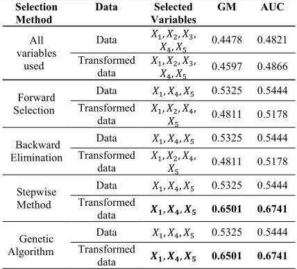
The comparison results of the four selection methods are presented in Table 13. The classification performances for testing dataset also summarized.
Table 13. The Performance Comparison of Variable Selection Methods in Discriminat Analysis (90:10 split)
Selection Method
Data Selected Variables
GM AUC
All variables
used
Data 𝑋 , 𝑋 , 𝑋 ,𝑋 , 𝑋 0.4478 0.4821
Transformed
data 𝑋 , 𝑋 , 𝑋 ,𝑋 , 𝑋 0.4597 0.4866
Forward Selection
Data 𝑋 , 𝑋 , 𝑋 0.5325 0.5444 Transformed
data 𝑋 , 𝑋 , 𝑋 ,𝑋 0.4811 0.5178
Backward Elimination
Data 𝑋 , 𝑋 , 𝑋 0.5325 0.5444 Transformed
data 𝑋 , 𝑋 , 𝑋 ,𝑋 0.4811 0.5178
Stepwise Method
Data 𝑋 , 𝑋 , 𝑋 0.5325 0.5444 Transformed
data 𝑿𝟏, 𝑿𝟒, 𝑿𝟓 0.6501 0.6741
Genetic Algorithm
Data 𝑋 , 𝑋 , 𝑋 0.5325 0.5444 Transformed
data 𝑿𝟏, 𝑿𝟒, 𝑿𝟓 0.6501 0.6741
From Table 13, we can see that variables selected from forward selection method, backward elimination, stepwise method and genetic algorithms are different, both from data that has met the assumptions and those that violate the assumptions. In addition, it was found that the highest AUC (0.6741) and GM (0.6501) are obtained from Stepwise method and Genetic Algorithm, with the selected variables are
𝑋 , 𝑋 and 𝑋 .
After obtaining the selected variables, then genetic algorithm is used to estimate the parameters of the discriminant function that can minimize misclassification. The steps taken to optimize parameter estimation are the same as genetic algorithms for variable selection, the difference is in the chromosome representation in initialization step.
The first step of genetic algorithm for parameter estimation is to initiate chromosomes with the total of 100 where each chromosome consists of 15 genes. One of the chromosomes is a solution (parameter estimate) obtained from discriminant function analysis. Figure 5 shows one example of chromosome representation for linear discriminant function analysis.
-11.3 0.7 ⋯ 0.9 .. .. 16.6 -0.01 ⋯ 0.64
𝛼 𝑊 ⋯ 𝑊 𝛼 𝑊 ⋯ 𝑊
[image:7.612.307.525.666.696.2]𝑦 𝑦
1852 The classification results for data partition 90:10 using four selection methods followed by genetic algorithm for parameter estimation are summarized in Table 14, both for data where the assumptions are not met and the second for transformed data where the assumptions are met.
Table 14: Classification Performance of Hybrid DA-GA for Data Partition 90:10
Selection Method
Data Transformed
Data
GM AUC GM AUC
No Selection 0.7071 0.7316 0.7194 0.7321
Forward
Selection 0.6049 0.6161 0.6874 0.7098 Backward
Elimination 0.6049 0.6161 0.6874 0.7098 Stepwise
Method 0.6049 0.6161 0.7530 0.7321 Genetic
Algorithm 0.6049 0.6161 0.7530 0.7321
It was shown that the best GM and AUC are obtained from Stepwise Method and Genetic Algorithm as selection methods followed by genetic algorithm for parameter estimation. The selected variables are 𝑋 , 𝑋 and 𝑋 so the best Hybrid Genetic Algorithm- Discriminant Analysis model is as follows.
𝑍 15.08 0.0721𝑋 2.6153𝑋 0.8699𝑋 𝑍 2.741 0.056𝑋 0.514𝑋 0.9877𝑋 𝑍 0.733 0.0389𝑋 4.0537𝑋 0.7328𝑋
The values of the discriminant function are the contribution values of each variable to classification. The coefficient with a positive value means the chance of an observation entering a class is increasing, while the coefficient with a negative value means the chance for an observation to enter a class is decreasing.
The same analysis is performed on the Data Partition 80:20. The assumption testing indicates that multivariate normal assumptions and homogeneous variance-covariance are violated so that transformation needs to be done. The Box-cox transformation value for data partition 80:20 are similar to transformation in data partition 90:10. After the assumptions are met then variable selection is done. The results of the variable selection from the four methods are summarized in Table 15.
Table 15: The Performance Comparison of Variable Selection Methods in Discriminant Analysis (80:20 split)
Selection
Method Data
Selected
Variables GM AUC
All variables
used
Data 𝑋 , 𝑋 , 𝑋 ,
𝑋 , 𝑋 0.4331 0.5468
Transformed data
𝑋 , 𝑋 , 𝑋 ,
𝑋 , 𝑋 0.5150 0.5781
Forward Selection
Data 𝑋 , 𝑋 , 𝑋 ,𝑋 0.4331 0.5468
Transformed
data 𝑋 , 𝑋 , 𝑋 ,𝑋 0.5150 0.5781
Backward Elimination
Data 𝑋 , 𝑋 , 𝑋 ,
𝑋 0.4331 0.5468 Transformed
data
𝑋 , 𝑋 , 𝑋 ,
𝑋 0.5150 0.5781 Stepwise
Method
Data 𝑋 , 𝑋 , 𝑋 0.4746 0.6093 Transformed
data 𝑋 , 𝑋 , 𝑋 0.5837 0.6584
Genetic Algorithm
Data 𝑋 , 𝑋 , 𝑋 0.6050 0.6383 Transformed
data 𝑋 , 𝑋 , 𝑋 0.5837 0.6584
[image:8.612.94.294.199.324.2]Table 15 shows that different selection methods can yield on different variables. Genetic Algorithm performs best in classifying patients risk based on GM. Based on AUC, Stepwise and Genetic Algorithm methods perform best. Table 16 presents the results of the classification performance from the four methods for Data Partition 80:20 followed by the step of optimizing the parameter estimation using Genetic Algorithm.
Table 16: Classification Performance of Hybrid DA-GA for Data Partition 80:20
Selection Method
Data Transformed
Data
GM AUC GM AUC
No Selection 0.7339 0.7500 0.6804 0.6853 Forward
Selection 0.7477 0.7679 0.7477 0.7210 Backward
Elimination 0.7477 0.7679 0.7477 0.7210 Stepwise
Method 0.7339 0.7522 0.7031 0.7321 Genetic
Algorithm 0.6839 0.7187 0.7031 0.7321
It is shown in Table 16 that for data partition 80:20, forward selection and backward elimination hybridized with GA in parameter optimization can produce highest GM and AUC that are 74.77% and 76.79% respectively. The selected variables are 𝑋 , 𝑋 , 𝑋 and 𝑋 . The best hybrid Discriminant Analysis–Genetic Algorithm model is
[image:8.612.310.526.460.576.2]1853 7.3 Naïve Bayes Analysis
The initial step in Naïve Bayes analysis is to calculate the prior probability value. In the partition data 90:10, the training data consists of 70 observations in class II, 59 observations in class III, 36 observations in class IV and 10 observations in class V. Prior probability values for Data Partition 90:10 are presented in Table 17.
Table 17: Prior Probability for Data Partition 90:10
Class Probability II 0.4000 III 0.3371 IV 0.2058 V 0.0571
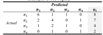
[image:9.612.309.533.115.244.2]Next, calculate the mean and standard deviation of each variable in each category. After that, the partial probability values are calculated using the Gauss density function as in equation (12) and then calculate the posterior probability values, which are then used to determine the prediction results on the testing data. Predictions results are then compared to the actual data.
Table 18: Classification Performance of Naïve Bayes Classifier (90:10 split)
Predicted
𝝅𝟏 𝝅𝟐 𝝅𝟑 𝝅𝟒 𝒏𝒍
Actual
𝜋 6 1 1 0 8
𝜋 2 4 0 1 7
𝜋 1 2 1 0 4
𝜋 0 1 0 1 2
From the results in Table 18, then calculate the miss classification value using expanding geometric-mean (GM) and Area Under Curve (AUC) for both data and transformed data. Similar steps are applied for transformation data and Data partition 80:20. Based on Table 19, it can be seen that by using GM, it is possible to obtain 0% classification accuracy of testing data. These occurs because there are one or more classes in predicted data that have no members.
In addition, the highest GM values for Data Partition 90:10 and 80:20 are obtained from data where the assumptions are met and the selection methods used are Stepwise methods and Genetic algorithm, which are 50.87% and 64.6 % respectively. The same conclusion is obtained from AUC comparison as presented in Table 20.
Table 19: Classification Performance of Naïve Bayes based on Geometric Mean (GM)
Selection Method
90:10 80:20
Data Tranformed Data Data Transformed Data
No Variable
Selection 0.4811 0 0.5087 0
Forward
Selection 0 0 0.5287 0
Backward
Elimination 0 0 0.5287 0
Stepsiwe
Method 0 0.5087 0.5087 0.6460
Genetic
[image:9.612.307.535.280.408.2]Algorithm 0 0.5087 0.4370 0.6460
Table 20: Classification Performance of Naïve Bayes based on Area Under Curve (AUC)
Selection Method
90:10 80:20
Data Tranformed Data Data Transformed Data No
Selection 0.5178 0.0952 0.5339 0.0975
Forward
Selection 0.3404 0.0952 0.5284 0.0975
Backward
Elimination 0.3404 0.0952 0.5284 0.0975
Stepsiwe
Method 0.3404 0.5339 0.5339 0.6069
Genetic
Algorithm 0.3404 0.5339 0.4841 0.6069
7.4 Comparison between Hybrid Genetic Algorithm-Discriminant Analysis and Naïve Bayes
[image:9.612.94.291.396.464.2]After obtaining the value of GM and AUC from every method, a comparison is carried out
.
Table 21: Overall Comparison
Method Parti tion Data Variables Selected GM Classification AUC
Discriminant Analysis
90:10 Data 𝑋 , 𝑋 , 𝑋 0.5325 0.5444
Transf 𝑋 , 𝑋 , 𝑋 0.6501 0.6741
80:20 Data 𝑋 , 𝑋 , 𝑋 0.6050 0.6383
Transf 𝑋 , 𝑋 , 𝑋 0.6584 0.6584
Hybrid DA-GA
90:10 Data
𝑋 , 𝑋 , 𝑋 ,
𝑋 , 𝑋 0.7071 0.7316
Transf 𝑋 , 𝑋 , 𝑋 0.7530 0.7321
80:20
Data 𝑋 , 𝑋 , 𝑋 ,
𝑋 0.7477 0.7679
Transf 𝑋 , 𝑋 ,
𝑋 , 𝑋 0.7477 0.7210
Naïve
Bayes 90:10 Data 𝑋 , 𝑋 , 𝑋 𝑋 , 𝑋 0.4811 0.5178
Transf 𝑋 , 𝑋 , 𝑋 0.5087 0.5339
80:20 Data 𝑋 , 𝑋 , 𝑋 0.5287 0.5339
[image:9.612.306.545.505.700.2]1854 Table 20 shows that highest values of GM and AUC are 74.77% and 76.79% respectively, obtained from hybrid genetic algorithm- discriminant analysis. The selected variables
are 𝑋 , 𝑋 , 𝑋 and 𝑋 .
8.CONCLUSION
It can be concluded that:
1. From the data, there were no patients that classified into class I, 40% patients are in class II, 34% in class III, 20% in class IV and 6% are in class V.
2. The variable that can be used to discriminate patients risk in Data Partition 90:10 and 80:20 are different. In data partition 90:10 and 80:20 when the assumptions are met, the variables that selected from forward selection and
backward elimination are 𝑋, 𝑋 , 𝑋 , and 𝑋 , while stepwise method and Genetic Algorithm select 𝑋, 𝑋 and 𝑋 . The same selected variables are produced from forward selection, backward elimination, stepwise method and Genetic Algorithm for Data Partition 90:10 when the assumptions are violated. For Data Partition 80:20 when the assumptions are violated, forward selection and backward elimination gives the same result that is 𝑋 , 𝑋,
𝑋 and 𝑋 are selected; while stepwise method selects 𝑋, 𝑋 , and 𝑋 and Genetic Algorithm selects 𝑋, 𝑋, and 𝑋 .
3. Optimization of parameter estimation using genetic algorithm in discriminant analysis gives better classification result than discriminant analysis, both for data when assumption is met or not.
4. The highest GM and AUC are 74,77% and 76,79%, obtained from Hybrid Genetic Algorithm-Discriminant Analysis with the selected variables are 𝑋 , 𝑋 , 𝑋 and 𝑋 .
5. Multi-class Classification performance using GM and AUC give the same result that is the Hybrid Genetic Algorithm-Discriminant Analysis produces better classification performance than Naïve Bayes.
Further study can be carried out using simulation data with various characteristics of the data, so that it can be known the performance of the genetic algorithm for variable selection and parameter estimation based on simulated data characteristics.
ACKNOWLEDGEMENT
The authors gratefully thank the Ministry of Research, Technology and Higher Education, Republic of Indonesia and Institut Teknologi Sepuluh Nopember Surabaya Indonesia for the financial support under “Penelitian Fundamental”.
REFERENCES
[1] Depkes R.I. (2002). Pedoman Pemberantasan Penyakit Infeksi Saluran Pernafasan Akut untuk Penanggulangan Pneumonia pada Balita dalam Pelita VI. Jakarta: Dirjen PPM & PLP.
[2] Badan Penelitian dan Pengembangan Kesehatan. (2013). Riset Kesehatan Dasar : RISKESDAS 2013. Jakarta: Kementrian Kesehatan Republik Indonesia.
[3] Tierney, L. M., McPhee, S. J., & Papadakis, M. A. (2002). Diagnosis dan Terapi Kedokteran (Penyakit Dalam). (G. Abdul, Y. T. Sofyatul, Erlina, & Isnatin, Trans.) Jakarta: Salemba Medika.
[4] Perhimpunan Dokter Paru Indonesia. (2003).
Pneumonia Kominiti: Pedoman Diagnosis & Penatalaksanaan di Indonesia. Jakarta: Perhimpunan Dokter Paru Indonesia.
[5] Gradianta, R. D., & Irhamah. (2014).
Klasifikasi Pasien Penderita Diabetes Melitus Tipe Dua Menggunakan Metode Analisis Diskriminan Hybrid Algoritma Genetika.
Jurnal Sains dan Seni ITS, Vol 3 no 2. Surabaya: Institut Teknologi Sepuluh Nopember.
[6] Kurnianto, I. P., & Irhamah. (2016). Forest Type Classification Based Spectral Characteristics using Hybrid Discriminant Analysis and Genetic Algorthm. Proceedings of the 6th Annual Basic Science International Conference (pp. 401-405). Malang: Brawijaya University.
[7] Islam, S., & Islam, R. (2011). Modeling Spammer Behavior: Artificial Neural Network vs. Naïve Bayesian Classifier.
Artificial Neural Networks, Chi Leung Patrick Hui. IntechOpen. DOI: 10.5772/16002. [8] Nayak, A., & Natarajan, D. S. (2016).
1855 [9] Johnson, R. A., & Winchern, D. W. (2007).
Applied Multivariate Statistical Analysis (6th ed.). New Jersey: Pearson Prentice Hall [10]Hair, J., Black, W., Barbin, B. J., & Anderson,
R. (2010). Multivariate Data Analysis 7th Edition. New Jersey: Pearson Prentice Hall. [11]Mardia, K.V. (1970) Measure of Multivariate
Skewness and Kurtosis with Applications.
Biometrika, 57(3):519-530
[12]Dillon, W. R., & Metthew, G. (1984).
Multivariate Analysis Methods and Application. United States of America: John Wiley & Sons, Inc.
[13]Gen, M., & Cheng, R. (1997). Genetic Algorithms and Engineerung Design. New York: John Wiley & Sons, Inc.
[14]Irhamah & Ismail, Z. (2009). A Breeder Genetic Algorithm for Vehicle Routing Problem with Stochastic Demands. Journal of Applied Sciences Research, 5(11): 1998-2005. [15]Sivanandam, S. N., & Deepa, S. N. (2008).
Introduction to Genetic Algorithms. New York: Springer-Verlag Berlin Heidelberg. [16]Wu, X., & Kumar, V. (2009). The Top Ten
Algorthms in Data Mining. New York: CRC Press.
[17]Sudoyo, A. W., Setiyohadi, B., Alwi, I., Simadibrata, M., &Setiati , S. (2009). Buku Ajar Imu Penyakit Dalam Jilid II Edisi V.