Solution Algorithm for Transportation Problem

(1)

Solution Algorithm for Transportation Problem

Darius P.B. Yusuf

1

,Bello S. Adekunle

2

, Koko K.M.

3

1_{Mathematics Department, Kaduna State College of Education Gidan Waya Kafanchan, Nigeria.Email:}_{[email protected]} 2_{Mathematics Department, Nasarawa State University, Nigeria}

3_{Department of General Studies Education, Federal College of Education Zaria, Nigeria}

Abstract

The proposed solution algorithm for transportation problem is considered in this paper.The objective in a transportation problem is to fully satisfy the destination requirements within the operating production capacity constraints at the minimum possible cost. Whenever there is a physical movement of goods from the point of manufacturer to the final consumers through a variety of channels of distribution (wholesalers, retailers, distributors etc.), there is a need to minimize the cost of transportation so as to increase profit on sales. The data obtained were modelled as a special Linear Programming problem. The MATLAP software is used to generate an optimal solution and the transportation problem was formulated and initial feasible solution was obtain using VAM, the solution obtained was tested for optimality using MODI.The model is useful for making strategic decisions involved in selecting optimum transportation routes so as to allocate the production of various plants to several warehouses or distribution centers.

Keywords

:

Objective function, Constraint, Transportation problem, Optimality test, Vogel’s

approximation Method.

1.

Introduction

:The transportation problem (TP) is an important Linear Programming (LP) model that arises in several contexts and has deservedly received much attention in literature.

The transportation problem is probably the most important special linear programming problem in terms of relative frequency with which it appears in the applications and also in the simplicity of the procedure developed for its solution. The following features of the transportation problem are considered to be most important.

The TP were the earliest class of linear programs discovered to have totally unimodular matrices and integral

extreme points resulting in considerable simplification of the simplex method.

The study of the TP laid the foundation for further theoretical and algorithmic development of the minimal cost network flow problems. Transportation problem is famous in operation research for its wide application in real life. This is a special kind of the network optimization problems in which goods are transported from a set of sources to a set of destinations subject to the supply and demand of the source and destination, respectively, such that the total cost of transportation is minimized.

The basic transportation problem was originally developed by (Hitchcock 1941) [1]. Aashtiani and Mohammadian (2009) [2] indicated thatthe transportation solution problem can be found with a good success in the improving the service quality of the public transport systems. Ahmed et al (2016) [3] investigated TP with a new approach named allocation table method (ATM) for finding an initial basic feasible solution of transportation problems, efficiency of allocation table method has also been tested by solving several number of cost minimizing transportation problems and it is found that the allocation table method yields comparatively a better result. The BCM obtained the optimal solution or the closest to optimal solution with a minimum computation time. As well as, using BCM will reduces the complexity with a simple and a clear solution manner which is easily used on different area for optimization problems,(Hlayel and Alia 2012) [4].

Minimization of transportation time is a great concern of the transportation problems like the cost minimizing transportation problems. In this writing, a transportation algorithm is developed and applied to obtain an Initial Basic Feasible Solution (IBFS) of transportation problems in minimizing transportation time. The developed method has also been illustrated numerically to test the efficiency of the method where it is observed that the proposed method yields a better result, (Ahmed et al 2015) [5].

2. Model Formulation of Problem:

The transportation problem deals with a situation in which a single product is to be transported from several sources (also call origin, supply or capacity centers) to several sinks (also called destination, demand or requirement centers). In general, let there

be m sources

s s

1, 2,

...

,

s

m

having

a i

i

(



1, 2,..., )

m

units of supplies or capacity respectively to be transported

(2)

cost of shipping one unit of the commodity from source

i

to destination

j

for each route. If

x

_ij represent the number of units shipped per route from source

i

to destination

j

then the problem is to determine the transportation schedule so as to minimize the total transportation cost satisfying supply and demand conditions. Mathematically, the problem may be stated as follows:

Minimize (total cost) Z =

1 1

m n

ij ij

i j

c x

 



……….……...……… (1)

Subject to the constraints

1 ,

n

ij

i

x

a





i



1, 2,...,

m

(Supply constraints)………....… (2)

1

,

n

ij j

i

x

b





j



1, 2,...,

n

(Demand constraints)……...……….…… (3)

And

x

ij



0

for all

i

and

j

The transportation problem can be described using linear programming mathematical model and usually it appears in a transportation tableau.

The model of a transportation problem can be represented in a concise tabular form with all the relevant parameters.

The transportation tableau (A typical TP is represented in standard matrix form), where supply availability (ai) at each source is

shown in the far right column and the destination requirements (bj) are shown in the bottom row. Each cell represents one route.

The unit shipping cost (Cij) is shown in the upper right corner of the cell, the amount of shipped material is shown in the center

of the cell. The transportation tableau implicitly expresses the supply and demand constraints and the shipping cost between each demand and supply point.

VOGEL’S APPROXIMATION METHOD (VAM)

VAM is an improved version of the least-cost method that generally, but not always, produces better starting solutions. VAM is based upon the concept of minimizing opportunity

(Or penalty) costs. The opportunity cost for a given supply row or demand column is defined as the difference between the lowest cost and the next lowest cost alternative. This method is preferred over the methods discussed above because it generally yields, an optimum, or close to optimum, starting solutions. Consequently, if we use the initial solution obtained by VAM and proceed to solve for the optimum solution, the amount of time required to arrive at the optimum solution is greatly reduced. The steps involved in determining an initial solution using VAM are as follows: The steps involved in determining an initial solution using VAM are as follows:

Step1. Write the given transportation problem in tabular form (if not given).

Step2. Compute the difference between the minimum cost and the next minimum cost corresponding to each row and each column which is known as penalty cost.

Step3. Choose the maximum difference or highest penalty cost. Suppose it corresponds to the ith row. Choose the cell with minimum cost in the ith row. Again if the maximum corresponds to a column, choose the cell with the minimum cost in this column.

Step4. Suppose it is the (i, j)th cell. Allocate min (ai, bj) to this cell. If the min (ai, bj) = ai, then the availability of the ith origin

is exhausted and demand at the jth destination remains as

bj-ai and the ith row is deleted from the table. Again if min (ai, bj) = bj, then demand at the jth destination is fulfilled and the

availability at the ith origin remains to be ai-bj and the jth column is deleted from the table.

Step5. Repeat steps 2, 3, and 4 with the remaining table until all origins are exhausted and all demands are fulfilled. - Method is based on the concept of penalty cost or regret.

- A penalty cost is the difference between the largest and the next largest cell cost in a row (or column). - In VAM the first step is to develop a penalty cost for each source and destination.

- Penalty cost is calculated by subtracting the minimum cell cost from the next higher cell cost in each row and column.

(3)

1. Determine the penalty cost for each row and column. 2. Select the row or column with the highest penalty cost.

3. Allocate as much as possible to the feasible cell with the lowest transportation cost in the row or column with the highest penalty cost.

4. Repeat steps 1, 2, and 3 until all rim requirements have been met Let Y1 and Y2=plant site

Xij = the units shipped in trucks from plant i to construction sites j

Using the transportation cost data, the weekly transportation cost in thousands of naira is written as:

Minimize

11 12 13 14 15 16 17

21 22 23 24 25 26 27

50

85

90

30

50

60

40

100

85

50

70

80

90 x

x



Consider capacity constraint

11

12

13

14

15

16

17

21

22

23

24

25

26

27

96

48 x

x

      

Demand constraint

11 21

12 22

13 23

14 24

15 25

16 26

17 27

22

28

18

15

18

19

24 x

x





























0

ij

x



For all

i

and

j

3. Solution of the Problem: Matrix Solution of Problem

F=[50 85 90 30 50 60 40 100 85 50 70 80 80 90];

A=[1 1 1 1 1 1 1 0 0 0 0 0 0 0;0 0 0 0 0 0 0 1 1 1 1 1 1 1;1 0 0 0 0 0 0 1 0 0 0 0 0 0;0 1 0 0 0 0 0 0 1 0 0 0 0 0;0 0 1 0 0 0 0 0 0 1 0 0 0 0;0 0 0 1 0 0 0 0 0 0 1 0 0 0;0 0 0 0 1 0 0 0 0 0 0 1 0 0;0 0 0 0 0 1 0 0 0 0 0 0 1 0;0 0 0 0 0 0 1 0 0 0 0 0 0 1];

b=[96 48 22 28 18 15 18 19 24]; x=A\b

(4)

0 15.0000 0 19.0000 -14.0000

Z = #9100

4. Vogel’s Approximation Method Solution

TABLE 1: The VAM Table

A B C D E F G CAPACITY

Y1 50 85 90 30 50 60 40 2880

Y2 100 83 50 70 80 80 90 1440

DEMAND 660 840 540 450 540 570 720 4320

Table 2: The VAM penalty cost

A B C D E F G CAPACITY Diff Y1 50 85 90 30 50 60 40 96 10

Y2 100 83 50 70 80 80 90 48 20

DEMAND 22 28 18 15 18 19 24 144 Difference 50 2 40 40 30 20 50

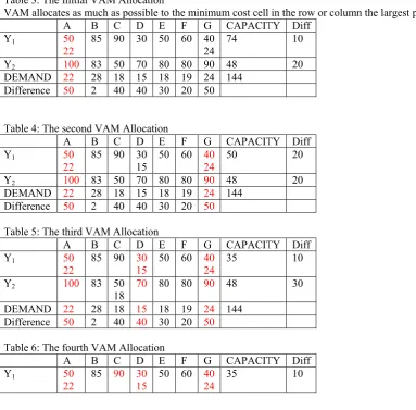
Table 3: The Initial VAM Allocation

VAM allocates as much as possible to the minimum cost cell in the row or column the largest penalty cost. A B C D E F G CAPACITY Diff

Y1 50

22

85 90 30 50 60 40 24

74 10

Y2 100 83 50 70 80 80 90 48 20

Table 4: The second VAM Allocation

A B C D E F G CAPACITY Diff

Y1 50

22 85 90 30 15 50 60 40 24 50 20

Y2 100 83 50 70 80 80 90 48 20

Table 5: The third VAM Allocation

Y1 50

22

85 90 30 15

50 60 40 24

35 10

Y2 100 83 50

18 70 80 80 90 48 30 DEMAND 22 28 18 15 18 19 24 144

Difference 50 2 40 40 30 20 50

Table 6: The fourth VAM Allocation

Y1 50

22

85 90 30 15

50 60 40 24

(5)

Y2 100 83 50

18 70 80 80 90 30 0

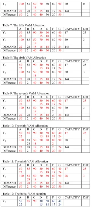
Table 7: The fifth VAM Allocation

Y1 50

22

85 90 30 15

50 18

60 40 24

17 25

Y2 100 83 50

18 70 80 80 90 30 3

Table 8: The sixth VAM Allocation

A B C D E F G CAPACITY diff

Y1 50

22 85 90 30 15 50 18 60 17 40 24 17 25

Y2 100 83 50

18

70 80 80 90 30 3

Table 9: The seventh VAM Allocation

Y1 50

22 85 90 30 15 50 18 60 17 40 24 17 25

Y2 100 83 50

18

70 80 80 2

90 30 3

Table 10: The eight VAM Allocation

Y1 50

22 85 90 30 15 50 18 60 17 40 24 17 25

Y2 100 83

28 50 18 70 80 80 2 90 28 3

Table 11: The ninth VAM Allocation

Y1 50

22 85 90 30 15 50 18 60 17 40 24 17 25

Y2 100 83

28 50 18 70 80 80 2 90 28 3

Table 12: The initial VAM solution

Y1 50

(6)

Y2 100 83

28 50 18 70 80 80 2 90

DEMAND Difference

5022 3015 5018 6017 4024 8328 5018 802 7814

Z







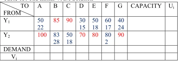
5. Application of Modified Distribution Method to Test Optimality of Initial Solution

STEP 1

The numbers of occupied cells are m+n-1 = 2 + 7 – 1 = 8 implies that initial solution is non-degenerate. Thus an optimal solution can be obtained. The total transportation cost associated with this solution is #7,814,000.00

Table 13: The Initial VAM Solution TO

FROM A B C D E F G CAPACITY Ui

Y1 50

22 85 90 30 15 50 18 60 17 40 24

Y2 100 83

28 50 18 70 80 80 2 90

DEMAND Vj

STEP 2

In order to compute the values of Ui(i=1,2) and Vj(j=1,2,…,7) for each occupied cell we arbitrarily assign V6=0

Given V6=0, U1 and U2 can be computed immediately by using the relation

Ui + Vj = Cij (unit transportation cost for cell ij) for occupied cells as shown below:

(7)

6

16 1 6 1

26 2 6 2

11 1 1 1

14 1 4 4

15 1 5 5

16 1 6 6

17 1 7 7

22 2 2 2

23 2 3 3

26 2 6 6

0

60

80 50 60

10 30 60

30 50 60

10 60 60

0 40 60

20 83 80

3 50 80

30

80 V

C

U

V

U

C

U

V

U

C

U

V

C

U

V

C

U

V

C

U

V

C

U

V

C

U

V

C

U

V

C

U

V























 











 











 





















 





















 











80 

0

STEP 3

The opportunity cost for each of the unoccupied cells is determined by using the relation Dij = Cij – (Ui + Vj) and is shown below:

12

1

2

13

1

3

21

2

1

24

2

4

25

2

5

27

2

7 (

) 85 (60 3) 22

(

) 90 (60 30) 60

(

) 100 (80 10) 30

(

) 70 (80 30) 20

(

) 80 (80 10) 10

(

) 90 (80 20) 30

D

C

U V

D

C

U V

D

C

U V

D

C

U V

D

C

U V

D

C

U V







 

 







 







 









 









 









 





According to the optimality criterion for cost minimizing transportation problem, the current solution is optimal, since the opportunity cost for unoccupied cells are all positive.

6. Result and Discussion

The above transportation problem was solved using VAM and optimality test was carried out using MODI, the result obtained shows that the initial VAM solution is optimal.

The Matlab solution using Gaussian method shows that the minimum total transportation cost is #9,100,000.00

The values for the basic variables show the optimal amounts to ship over each route. The logistics manager should follow the following distribution list if want to optimize the distribution:

(8)

Ship 15 trucks of product from Y1 to D.

Ship 18 trucks of product from Y1 to E.

Ship 17 trucks of product from Y1 to F.

Ship 24 trucks of product from Y1 to G.

Ship 28 trucks of product from Y2to B.

Ship 18 trucks of product from Y2 to C.

Ship 2 trucks of product fromY2 to F.

7. Conclusion

The transportation cost is an important element of the total cost structure for any business, the transportation problem was formulated and initial feasible solution was obtain using VAM, the solution obtained was tested for optimality using MODI. The computational results provided the minimal total transportation cost and the values for the decision variables for optimality. Optimum solutions provided the valuable information such as analysis for industries to make optimal decisions through the use of this mathematical model (Transportation Model), the model can identify easily and efficiently plan out transportation problem.

6. References

[1] Hitchcock, F.L. (1941), the Distribution of a Product from Several Sources to Numerous Localities. Journal of Mathematicsand Physics, 20, 224-230.

[2] Amir, S., H.Z. Aashtiani and K.A. Mohammadian, (2009), A Short-term Management strategy for Improving transit network efficiency. Am. J. Applied Sci., 6: 241-246.

[3] Ahmed, M.M., Khan, A.R., Uddin, Md.S. and Ahmed, F. (2016), a New Approach to Solve Transportation Problems.

Open Journal of Optimization, 5, 22-30.

[4] Abdallah A. Hlayel, Mohammad A. Alia (2012), solving transportation problems using the best candidate’s method,

Computer Science & Engineering: An International Journal (CSEIJ), Vol.2, No.5

[5] Ahmed, M.M., Islam, Md.A. Katun, M., Yesmin, S. and Uddin, Md.S. (2015) New Procedure of Finding an Initial Basic Feasible Solution of the Time Minimizing Transportation Problems. Open Journal of Applied Sciences, 5,