Dissertation zur Erlangung des Doktorgrades der Fakultät für Chemie und Pharmazie der Ludwig-Maximilians-Universität München
TRANSLATIONAL, ORIENTATIONAL AND SPECTRAL DYNAMICS OF INDIVIDUAL MOLECULES IN NANO-STRUCTURED MATERIALS
STUDIED WITH SINGLE-MOLECULE-SPECTROSCOPY
Christian Hellriegel
aus
São Paulo, Brasilien
Erklärung
Diese Dissertation wurde im Sinne von §13 Abs. 3 bzw. 4 der Promotionsordung vom 29. Januar 1998 von Prof. Dr. Christoph Bräuchle betreut
Ehrenwörtliche Versicherung
Diese Dissertation wurde selbstständig, ohne unerlaubte Hilfe erarbeitet.
München, den 30.Juni 2005
(Unterschrift)
Index
1. Introduction 10
2. Theoretical Background 14
2.1. Host-Guest Materials 15
2.2. Fluorescence and SMS 28
2.2.1 Fluorescence 28
2.2.2. Single-Moelcule Spectroscopy 31
2.3. Diffusion 35
2.3.1 Macroscopic 35
2.3.2 Microscopic 37
3. Experimental Section 50
3.1. Microscopy Techniques 51
3.1.1 Confocal Microscopy 53 3.1.2 Widefield Imaging Microscopy 62
3.2. Analysis Programs 66
4. Results and Discussion 90 4.1. Characterization of Host-Guest Materials (ensemble) 91 4.2. Photostability of New Dyes for SMS 103 4.3. Orientational Distribution of Oxazine Dyes in AlPO4-5 109
4.4. Translational Diffusion of TDI in MCM41S Monoliths 114 4.5. Translational Diffusion of 9A1 in Sol-Gel Glass 117 4.6. Translational Diffusion of TDI Molecules in SBA-15 Films 130
4.7. Spectral Behavior of TDI in PMMA 137
4.8. Covalently bound Cy5 in MCM-41 148
5. Summary 158
6. Bibliographical Information 163
1. Introduction
The importance of materials in technology, science and everyday life is self-evident. Among promising materials for emerging applications (think of smart materials, medical diagnostics, nanoelectronic devices etc.) are the so-called host-guest materials, where a molecular species is incorporated as a guest into a solid host. Interesting hosts for the incorporation of guests (biomolecules, indicators, catalysts, fluorescent dyes, etc.) are, for example, inorganic micro- and mesoporous materials, which can be thought of as a well-defined system of nanometer-sized pores.[Davis02], [Wark03]
If such host-guest materials can be seen as a nanometer-sized system of pores in which the individual guest molecules may move, turn or perform a specific task, then it is of fundamental importance to observe and to understand the behavior of guest molecules in such a system.
The characterization of the behavior of fluorescent dye molecules in porous materials is the central topic of this thesis. The topic is addressed using single-molecule-spectroscopy (SMS) and microscopy techniques. It will be shown that SMS methods allow for a very thorough characterization of the behavior of dye molecules in the studied samples.
Since the first observations of individual molecules via fluorescence [Moerner89], [Orrit90], the SMS technique has developped to become a mature and established technique that can be used at room-temperature to investigate complex systems, like polymers, crystals, liquid solutions and biological samples [Basché96], [Nie97], [Xie98], [Tamarat00], [Rigler01]. Two recent reviews [Moerner02], [Kulzer04] cover the most recent developments in SMS. Apart from addressing interesting questions in material science [Gruber97], [Kulzer97], [Deschenes01], [Weston01], [Schuster02], it is clear that SMS can also be used as a powerful technique to answer biophysical questions
The first direct observation of the dynamics of individual fluorescent molecules in nanostructured porous materials were published in 2002 [Seebacher02] and were part of my diploma thesis. In the subsequent time, it was possible to expand the used SMS setup, to improve the data acquisition and evaluation so that presently it is not only possible to detect individual molecules in a nanostructured material but also to characterize their dynamical behavior at an unprecedented level of detail.
This thesis is subdivided into three main chapters (i.e. chapters 2, 3 and 4) followed by the summary, the bibliographical information and the appendix.
Chapter 2 covers the theoretical background and is subdivided into three sections. The first section describes the host structures, that is the inorganic porous materials used. The second section introduces fluorescence, as the measured quantity of the guest molecules, and describes the advantages of the SMS approach. The third section covers the topic of diffusion which is the main dynamical phenomenon observed.
Chapter 3 describes the experimental setup (confocal and widefield microscopes) and the evaluation programs used to analyze the data. The necessary theoretical background for the techniques is included in this chapter, in the respective section. The emphasis of this chapter lies in the evaluation programs which were conceived and written in order to process the extensive amount of data produced by the microscopes. These programs are essential for the evaluation of data. Comparable or even suitable programs are not commercially available.
2. Theoretical Background
As outlined in the introduction, the main subject of the scientific investigations presented in this thesis is the dynamical behaviour of individual molecules incorporated as guests in a porous host material.
2.1. Host-Guest Materials
A host-guest material is any binary compound in which a molecular species, the guest, is incorporated into a solid matrix, the host. In a narrower definition a host-guest material also displays properties not present for the individual components and that result from the interplay between host and guest.[Langley99].
Figure 1: Schematical diagram illustrating the idea behind a host-guest material.
The broad variety of interplay possibilities between host and guest can be explored to generate interesting materials[Wark03], such as: novel pigments, phosphors, nonlinear optical materials[Caro94], micrometer-sized lasers[Schüth95], waveguides[Yang00], switchable membranes for size selective separation[Weh02], materials with controllable pore openings [Ban04], energy transfer materials[Gfeller98], sensors[Meinershagen99] and many more. There are numerous ways to combine host materials (polymers, glasses, porous materials, etc.) with guest species (dye molecules, catalytic complexes,
Inorganic porous materials have particularly appealing properties for the use as host materials: (a) The materials are mechanically, chemically and thermally stable. (b) Their structure allows an ordered incorporation of guests molecules creating well-defined spatial arrangements in the resulting host-guest material. (c) From the synthetic point of view the structure of the pores can be varied in size, interconnectivity and polarity. (d) Some of these materials can be thought of as a well-defined grid, or a system of pipes, for the ordered incorporation of functional guest molecules.
Despite the numerous applications and successful synthesis procedures leading to host-guest materials, there are many important open questions in the characterization of these materials. For example: (a) How do the guest molecules behave in the confined
environment? (b) What properties of the host and guest have an influence on this behaviour? (c) Can the behavior be influenced by external factors (e.g. light irradiation, addition of solvents)? (d) Over which range are the materials homogenous in their
properties? (e) How easily can molecules become incorporated into the materials? (f) Are the pores accessible to molecules coming from the outside? (g) Does the material degrade in any way? Etc.
2.1.1. Inorganic molecular sieves
'Molecular sieve' is the designation for any porous material capable of separating molecules due to the interplay between the pore-size and the molecular size, just like a sieve.[Szostak89] In this picture, the pore sizes of molecular sieves are comparable to the size of a molecule, i.e. between 0.1 and 10 nm. Inorganic porous materials such as sol-gel glasses, M41S-type materials and zeolites are typical molecular sieves. The materials investigated in this thesis are described in more detail below.
Sol-Gel-Glasses
The materials with the least ordered structure used in the presented studies are sol-gel-glasses (also called 'xerogels'). These amorphous, micro- and mesoporous silicas are widely used as hosts in technical applications because they are cheap and easy to prepare via a sol-gel synthesis [Brinker85] in a variety of physical forms, including powders, cast monoliths and spin-coated thin films. Sol-gel-glasses can be synthesized with a wide range of mean pore-diameters, from 0.5 nm to 200 nm and a wide range of specific surfaces from 100 to 1000 m2/g. The pores are interconnected, open to the exterior and can easily be loaded with gases, liquids or solids dispersed in a liquid.
Figure 2: Formation mechanisms of a sol-gel-glass. Sol-gel-glasses are formed from precursor particles or monomers, the sol, that condenses to form a gel. Further
condensation, aging and drying of the gel leads to the porous siliceous material, the sol-gel-glass. The gelation, aging and drying conditions affect the structure of the resulting porous material. Adapted from [Brinker85].
The advantages of using sol-gel-glasses to build host-guest materials are related to the simple synthesis procedure of the host material and the easy loading of the material with guest species. The high specific surface area, porosity and accessibility to molecules from the exterior of the solid body makes them, for example, ideal support materials for
catalysts.[Schwarz95] Furthermore, sol-gel-glasses are often used as model materials to study confinement effects, for example on solvation-dynamics [Baumann01],
The limitations of sol-gel-glasses in their use as host-matrices are directly related to their unspecific structure: The highly heterogenous pore architecture and the broad distribution of pore sizes makes sol-gel-glasses less suitable for materials that have to exhibit very specific effects related with the size and architecture of the pores, which for example are required in regioselective catalysis or molecular sieving with high size-specificity. In the same sense it is not possible to use these materials for the ordered incorporation of guests, as required e.g. in non-linear optical applications. The properties of the guests in such a disordered material will show a strong distribution or pronounced heterogeneities reflecting the various types, orientations and sizes of pores in which the guests may be incorporated. For example, processes and applications based on diffusion, like the suggested use of sol-gel glasses as a matrix for chromatography [McCalley05] or electrophoresis [Palmer02], are expected to show a pronounced heterogeneity.
Templated Mesoporous Materials
Templated mesoporous materials, like the group of M41S materials, represent the next level of structural organization of a molecular sieve. These amorphous porous silicas are synthesized via condensation, aging and drying of a gel formed by silica precursors (such as TEOS or TMOS) in the presence of a supramolecular structure-directing agent (SDA). [Kresge92], [Ying98] This supramolecular species, for example a surfactant forming a micellar liquid crystal, serves as a template around which the silica condenses forming the solid matrix.
evidence (in situ X-Ray diffractometry) indicating that the condensation of the solid matrix occurrs in a cooperative or concerted mechanism (fig. 3b). This seems to be the case in the synthesis using charged molecules as structure directing agent, and via evaporation induced self-assembly (EISA). [Grosso04], [Zhang02]
Figure 3: Suggested formation mechanism of templated mesoporous materials. a) Direct templating mechanism: The supramolecular structure (e.g. a micellar liquid crystalline phase) forms before condensation of the silica. b) Concerted or cooperative mechanism: The structure is formed as the silica condenses. Adapted from [Ying98]
The resulting pore topology formed by the supramolecular arrangement of the template may vary from micellar arrays to layered structures, as illustrated for M41S type materials in figure 4.
Figure 4: Different channel structures of M41S-Materials. The channel topology is a consequence of the organization of the supramolecular template formed in the synthesis. Shown here are three examples (from left to right): The pore architecture of MCM-41 results from a hexagonal array of micelles, the architecture of MCM-48 is based on a three-dimensial cubic arrangement of micelles and in MCM-50 the structure is formed on the basis of a layered structure of the template.
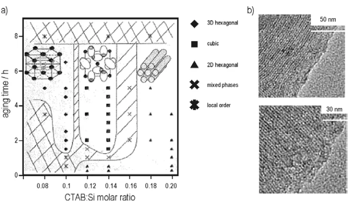
Figure 5: The formation of different structures depends on synthesis conditions. a) Phase diagram (aging time versus surfactant concentration) of CTAB Templated spin-coated films. Adapted from [Besson03] b) TEM images of spin-coated MCM-41 (CTAB template), corresponding to the 2D hexagonal phase in the phase diagram. The views in the micrographs are parallel to the substrate surface. Images from [Petkov04].
The short-range order of the pores - on the100 nm scale - can be characterized using X-ray diffraction techniques and transmission electron microscopy, TEM (e.g. fig. 5b). TEM images show that the pores, organized in hexagonal bundles, do not necessarily extend linearly over the entire body of the material. Instead, it is a common finding that the pores are arranged domains of a few 100 nm in size forming fingerprint motifs. The long-range order of the pores (in the order of a few µm) and the interconnectivity of the domains is presently not sufficiently well characterized.
Currently, some of the main challenges in the synthesis of these materials are: (a) To achieve an internal functionalization of the material, for example via covalent binding of dyes, catalysts and functional molecules, like cis-trans isomerizable molecules or
Zeolites, porosils and zeotype-structures
Crystalline porous solids like zeolites, porosils and zeotype-structures show the highest level of structural organization of a molecular sieve. A zeolite is commonly defined via its chemical structure, which consists of tetrahedral SiO44- and AlO45- subunits connected in a regular way. In a zeolite, the periodical arrangement of the chemical subunits forms crystallographically well-defined cages and pores, which are accessible to molecules from the exterior of the material. A porosil is similar to a zeolite in the sense that its structure can be derived from a zeolite structure, but it is composed exclusively of SiO2 units (e.g. Silicalite-1, SSZ-24, etc.). A zeotype-material is similar to a zeolite in the same sense, but is composed of different chemical subunits (e.g. AlPO4-5, CrAPO-5, etc.).
Figure 6: Typical examples for zeolite structures. From [ZeoliteAtlas05]
The structural arrangement of the aforementioned tetrahedral subunits results in typical types of pore openings, which can be classified according to the number of oxygen atoms present in the underlying ring structure, namely 12, 10 and 8 oxygen atoms. The
formation of the so-called supercages, which are nearly spherical voids with diameters in the nm-range, a well-known example for a zeolite with 1.3 nm supercages is faujasite (see fig. 6).
Zeolites are obtained in the laboratory by crystallisation of gels containing Al and Si sources in aqueous medium at temperatures in the range of 100-190 °C and autogenous pressure for several days or weeks. Besides Si and Al sources the reaction mixture can be prepared using other metal sources, and often also quaternary ammonium ions which direct the crystallisation to a specific crystal structure.[Corma04]
Zeolites are widely used as catalysts in technical applications, e.g. in catalytic cracking and Friedel-Crafts alkylation. Besides catalysis their well-defined structures can further be explored to generate host-guest materials with highly specific properties (sensors, solid lasers, etc.). The range of guest molecules that can be incorporated into a zeolite is, however, limited due to material's pore diameters. In a zeolite the pore diameter (or supercage opening) rarely exceeds 0.8 nm, making impossible the incorporation of more complex molecules, such as organic dye molecules which are often larger than 1 nm. It is possible, however, to form large molecular species in a zeolite supercage via a so-called ship-in-the-bottle synthesis[Domenech05],[Ricci04] or to encapsulate large molecules during synthesis [Ganschow01] - note that the encapsulation of large foreign species is likely to affect the structure of the material or to induce defects at the incorporation site.
Two important materials of this class, that have been studied in this thesis, are the zeotype AlPO4-5 (AFI) and the porosil Silicalite-1 (MFI).
AlPO4-5 (AFI): AFI is a zeotype material. Its structure (figure 7) is characterized by the
arrangement of AlO44- and PO43- tetrahedra that form hexagonally arranged
unidimensional channels of 0.73 nm in diameter (considering van-der-Waals radii). AFI can be synthesized in the form of large (µm to mm-sized) crystalline hexagonal prisms or rods. The large pore diameter, the unidimensional arrangement of the pores and the possibility to synthesize large crystalline bodies makes AFI an interesting host material for the ordered incorporation of organic dye molecules.
Figure 7: Structure of AlPO4-5 a) 3D-Structure b) 12-Ring dimensions. [ZeoliteAtlas05] and c) Transmission micrograph showing the typical habitus of the studied AFI crystals.
Silicalite-1: The porosil Silicalite-1 (MFI) can be synthesized in the form of µm-sized crystalline bodies with a well defined (usually coffin-shaped) morphology. MFI is an attractive material for technical applications because of the possibility to synthesise oriented films of MFI on various substrates [Xomeritakis99] (a defect free MFI film would, for example, act as a permselective membrane).
Its structure (figure 8) is characterized by the arrangement of two systems of pores of ca. 0.55 nm in diameter (considering van der Waals radii): (a) straight pores along [010] and (b) sinusoidal pores perpendicular to [010] interconnecting the pores (cf. figure 8a).
Figure 8: Structure of MFI. a) 3D-Structure of MFI b) 10-Ring dimensions c)
Transmission micrographs of MFI crystals showing its typical habitus. [Hellriegel03]
Summary: The most important properties of the host materials just discussed, with relevance for the studies presented in this thesis are resumed in the follwing table. The last column indicates in what study the host material has been used.
host-material pore-sizes (nm)
advantages limitations studied host-guest materials
sol-gel-glass 0.3-200 synthesis is easy, simple and cheap
a) heterogenous structure
b) distribution of pore sizes is very broad.
diffusion of VG5(dye) in sol-gel-glasses of different porosity
templated materials (M41S / SBA)
2-20 narrow distribution of pore-sizes, and well-defined architecture. a) synthesis difficulties b) long range (0.1-10 µm) order of pores not well-defined
a) diffusion of TDI(dye) in SBA-15 and MCM-41. b) Effect of different solvents on Cy5(dye) covalently bound to the pores of MCM-41
zeolites and zeotype- structures
0.3-0.8 crystalline
bodies a) small pores, b) synthesis of big defect-free crystals difficult
a) detection of defect structures on MFI coats. b) energy transfer between different dyes in AFI c) orientational
2.2. Fluorescence and Single-Molecule-Spectroscopy (SMS)
2.2.1 Fluorescence
Fluorescence can be described semi-classically by the interaction of light with a quantum mechanical system (cf. physical chemistry textbooks like [Moore76] or [Levine83]). In a simplified schematical energy diagram for organic fluorescent dye molecules, the
fluorescence occurrs as follows:
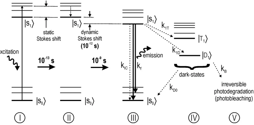
Figure 9: Schematical energy diagram illustrating the basic principles involved in fluorescence (dashed lines represent radiationless relaxation pathways).
Dynamics of Fluorescence: At room temperature a dye molecule rests in the lowest electronic state, the singlet S0. An incoming photon (with suitable energy and
dynamic (on the 10-12 s time-scale) Stokes shifts. Less probable steps from S1 are (a) the radiationless relaxation via internal conversion (IC), and (b) radiationless relaxations via dark-states, such as the triplet T1. From the dark-states the molecule may relax back to S0 from where a new excitation-relaxation cycle can begin again (IV→I). In the schematical diagram above, the transition probabilities to the involved states are expressed as
transition rates k. The ratio between the fluorescent rate kf and the sum of all relaxation rates, the fluorescence quantum yield φf, gives the probability that the relaxation from S1 will occur under emission of a photon:
φf = kf / kTOT (1)
With kTOT = (kf + kIC + k1T + k1D + k1D'...) increasing with additional radiationless relaxation mechanisms. Clearly, a good fluorescent dye molecule has a quantum yield near 1, and few interfering dark-states, or radiationless relaxation channels.
The best-understood and characterized dark-state is the triplet state T1.[McGlynn69] which can also be studied for specific fluorescent dye molecules [Kulzer99], [Fleury00], in these molecules the low triplet-rates k1T (between 10-4 and 10-5 s-1) do not effectively compete with the main relaxation channel of fluorescence. The typical life-time of the triplet in such molecules is in the order of a few µs. Some recent works covering the identification and the characterization of fluorescence dynamics involving other dark states are [Zondervan03], [Verberk02], [Renge02], [Zehetmayer02] and [Jung01b].
The End of Fluorescence / Photobleaching: In an idealized system the absorption-emission cycle would go on indeterminately. In real systems the molecule may undergo an irreversible reaction from one of the excited states (S1, T1, D, etc.) to form a non-fluorescing species. This last step in the duty-life of a fluorescent molecule is called 'photobleaching' (V in fig.9). The photobleaching mechanisms can be very complex, and few are presently understood in detail: The suggested mechanisms vary from reaction via the triplet state, or via other dark states (S2, T2, D', D'', etc.), from transient
Fluorescence Spectra: The relative positions of the states in the energy diagram above, result in the respective absorbtion and emission spectra. The typical room-temperature absorption and fluorescence spectrum of an organic dye molecule (TDI) is shown in fig.10 and consists of broadened emission bands resulting from the main (00) transition and transitions to vibronic states in S0 that may appear well or less well resolved depending on the molecule in question.
Figure 10: Typical absorption and emission spectrum of an organic fluorescent dye molecule (TDI in CHCl3; normalized spectra, excitation at 633 nm).
In an idealized system the absorption and emission lines should be as narrow as a few ten MHz, limited only by the uncertainty principle. However, in real systems and at room temperature the emission bands are broadened to some THz because of: (a) the homogenous broadening in which the underlying quantum mechanical systems are
2.2.2 Single-Moelcule Spectroscopy (SMS)
The essential task in single molecule spectroscopy (SMS) is to separate any signal, (e.g. fluorescence) from an individual molecule from the remaining signals of the sample (background light, fluorescence from other molecules, etc.). In principle tunneling microscopy (STM) [Binnig82],[Hofer03], force microscopy (AFM) [Binnig86],
[Giessibl03], and electron microscopy (SEM, TEM) [Fultz01], which can record images of a surface with a spatial resolution on the atomic scale, can also be counted to the SMS methods. More frequently, however, SMS is associated with optical emmission
spectroscopy and microscopy of individual fluorescing molecules (or particles such as nano-crystals), which can also be situated in the volume of a transparent sample. A number of reviews on SMS has been published in recent years. [Nie97], [Tamarat00], [Moerner02], [Barkai04], [Kulzer04]. The technique has gained considerable attention since the first experiments more than a decade ago; developping to become a mature technique employed in fields as diverse as biology [Rigler90], [Kinosita98], [Weiss99], [Kitamura99], [Seisenberger01] and material science [Gruber97], [Kulzer97],
[Deschenes01], [Weston01], [Schuster02]. SMS studies provide details that cannot be accessed by the conventional ensemble methods. The most important aspects of SMS, and these advantages, will be described in the following.
There are basically three strategies that can be followed in typical SMS measurements to isolate the emmission of individual molecules: (a) The spectral selection of fluorescence, which is typically carried out at liquid-helium temperatures, because the emission
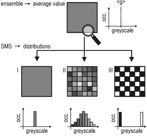
SMS resolves distributions: An SMS method has the capability of resolving individual properties of the investigated molecules, and thus has access to the distribution function of a studied property. This stands in contrast to conventional ensemble spectroscopy methods, in which properties are measured for an ensemble of molecules, and are perceived as a sum or an average from all contributions of all individual molecules.
Figure 11: Ensemble measurements give an average value for a measured property (here the greyscale value). SMS resolves the distribution of the values around the mean value. Note in case III that the mean value obtained in the ensemble measurement has no physical meaning.
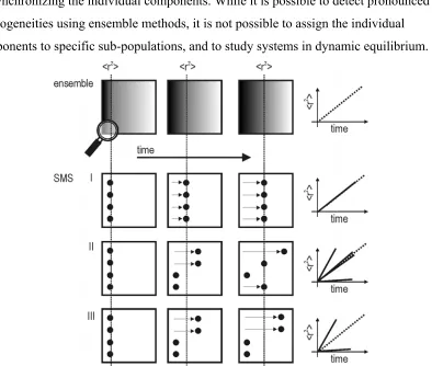
SMS resolves dynamics: In the same sense, the study of dynamics (e.g. diffusion) is more detailed in SMS. In an ensemble measurement it is only possible to study dynamics by synchronizing the individual components. While it is possible to detect pronounced heterogeneities using ensemble methods, it is not possible to assign the individual components to specific sub-populations, and to study systems in dynamic equilibrium.
Figure 12: Ensemble measurements fail to detect sub-populations in a dynamic
measurement (here, diffusion). The direct observation of individual molecules resolves sub-populations. Note in case III that the mean value obtained in the ensemble
measurement has no physical meaning.
sub-populations in case II. This kind of data is not available from ensemble measurements and allows for a thorough interpretation of the involved dynamics. It is possible to determine, for example, if the retardation of a particle during diffusion is caused by a specific mechanism (e.g. entering and escaping a bottle-neck trap). Furthermore it is possible to infer whether the effect is the same for all molecules or if two populations with differing diffusivities are separated but coexisting in the same sample.
SMS Summary: The SMS technique brings a series of advantages in the characterization of a sample because it detects the properties (e.g. fluorescence intensity, position,
fluorescence spectrum, polarization) of individual molecules and thus (a) resolves the distribution function of the studied property. This stands in contrast to an average value that can be obtained from a conventional measurement on an ensemble of molecules. (b) Using SMS it is possible to characterize dynamics in a high level of detail. (c) SMS also allows to observe and to characterize rare or extreme phenomena (on the flanks of a distribution curve) that would otherwise remain undetected in an ensemble measurement.
2.3. Diffusion
Diffusion is a fundamental phenomenon taking place on fields as diverse as biology, astronomy and communication sciences. In a very raw definition, diffusion can be seen as the dynamic spreading of any physical property, such as the amount of particles, heat, or information. In the following considerations, diffusion will be restricted to the transport of matter, and more specifically, to the diffusion of molecules, which is of obvious importance for applications based on porous materials: The working mechanisms and the performance of ion exchangers, catalysts, adsorbers and molecular sieves depend on the diffusion properties of the involved molecular species. Before turning to experimental considerations on how to observe and characterize diffusion, a compact introduction to the theoretical background of diffusion is given.
2.3.1. Macrsocopic Treatment of Diffsuion
Diffusion describes the movement of matter, or molecules in space and in time. It is possible to address the involved questions from a macroscopic (ensemble) and from a microscopic (particulate) perspective. In the macroscopic approach the amount of particles per volume is described by a concentration. Diffusion is then associated to the change of concentration with time and space. The theory of macroscopic diffusion is described by the Fickian equations (e.g. [Moore76]):
Jx,t = -D
( )
∂ ∂ x t x C , and
( )
( )
∂ ∂ = ∂ ∂ 2 2 , , x t x C D t t x C (2,3)
In words, the flux Jx,t of particles (along a spatial axis x and at a time t) is proportional to
this approach lies in the fact that it allows to predict the distribution of concentrations at any given time, just by knowing the initial concentrations and boundary conditions that define the diffusing system. Two relevant problems and the solutions for the differential equations (2,3) are given in the following (adapted from [Carlslaw59]):
a) Diffusion into a gaussian shaped, depleted region with a characteristic radius r and from a limited reservoir - e.g. dye diffusion into a photobleached spot, I(r,t) ~ C(r,t):
C (r,t) =
(
)
− Dt r Dt c 4 exp 4 2 3 0π (4)
b) Diffusion perpendicular to a plane source (along x) from an unlimited reservoir - e.g. dye uptake by a straight crystal boundary from solution, with I(x,t) ~ C(x,t):
C (x,t) =1- c0 erfc Dt x
4 (5)
Note: erfc(x) =
∫
− x w z 0 2 2 exp dz2.3.2. Microscopic Treatment of Diffusion
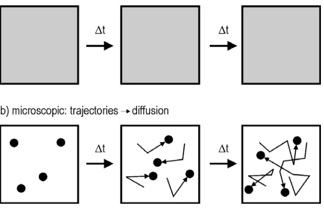
The macroscopic method, described above, has limitations. It is not sensitive towards different sub-populations or, more generally, to distributions of diffusional behaviours and depends strongly on the assumption of diffusion models. The experimentally observed behaviour is often difficult to characterize properly using the idealized ensemble models. Furthermore, the macroscopic approach using the Fickian diffusion equations will not work in the study of systems under equilibrium. In such systems the concentration gradient and consequently the net flux are zero, despite the fact that the molecules are actually diffusing (see fig.13).
In the microscopic approach, the characterization of diffusion is based on the observation of the movement of an individual diffusing particle (e.g. a fluorescent molecule). This method has a series of advantages over the macroscopic approach: (a) It is independent from any initial conditions (i.e. concentration gradients or other boundary conditions). The investigated system can thus be in equilibrium (see fig.13). (b) The evaluation based on the individual particle that makes up the ensemble contains information on the
distribution of diffusivities, which may vary spatially, or from particle to particle - the 'ensemble averaging' effect is supressed. Sub-populations and, in general, the
distributions of diffusional behaviours are resolved. (c) It is possible to resolve mechanistic details, or events such as adsorption / desorption, that take place during diffusion (transient traps).
The characterization of diffusion based on the observation of individual trajectories of a diffusing particle has to account for the statistical nature of diffusion.[Chandrasekhar43] This has two implications: First, a large number of individual trajectories has to be evaluated to allow for a proper description of the diffusional behaviour - this is
particularly important for the characterization of sub-populations and/or distributions of diffusional behaviours. Second, the physical interpretation of the diffusion process may become more complex, because the observation of individual trajectories reveal spatial and temporal heterogeneities not described by the simpler models of diffusion. While the measurements of individual trajectories is more difficult to accomplish experimentally, and while the analysis is more complex, the information gained from the analysis of individual trajectories adds a significant amount of quality to the obtained data.
Random walk: The isotropic random walk is the simplest mode of motion for a diffusing particle. A central result of the microscopic treatment of diffusion is that in a random walk, the mean square displacement of a diffusing particle, 〈r2(t)〉, follows a linear dependence with time:
〈r2(t)〉 = 4 Dt. (6)
Equation 6, the Einstein equation for a two-dimensional random walk, is the central equation in most diffusion studies.[Einstein05], [Einstein06] It can be shown that the diffusion coefficient D corresponds exactly to the macroscopic diffusion
coefficient.[Chadrasekhar43], [Berg93] In the microscopic model, the diffusion coefficient D describes the area that the particle explores per unit of time during its random walk.
Starting from a trajectory sampled in time intervals δt it is easy to calculate the mean square displacement 〈r2(t)〉 for every time lag t = nδt (n is the number of sample periods between two positions in the trajectory). In a random walk, every position of the
trajectory serves as a starting point for the analysis. With n steps in the trajectory the number of individual steps leading to a mean square displacement at a time lag t=1δt is n, the number of steps leading to a mean square displacement (MSD) at a time lag 2δt is n-1, for a time lag 3δt it is n-2 and so on. As a consequence the statistical error for the mean square displacement increases with observation time, as less steps are used to calculate the mean value. The diffusion coefficient D is obtained in a straightforward way via a linear regression for 〈r2(t)〉 versus time lag (see fig.14).
deviations from the linear behaviour in a 〈r2(t)〉 versus time plot. [Berg93], [Qian91], [Schmidt96], [Saxton97] and [Schütz97]. For some specific cases, it is possible to derive analytically a mathematical formula that describes the time dependence of the MSD. A small collection of such diffusion equations is given below (adapted from [Saxton97]):
nDt t
r2() =2 random walk in n-dimensions (7)
α
Dt t
r2() =4 anomalous 2D-diffusion (8)
( )
2 2(t) 4Dt Vtr = + 2D-diffusion with flow (9)
− − ≅ Dt r A A r t r C C 2 2 1 2
2( ) 1 exp 4 confined motion (10)
In these equations the mean-square displacements as a function of time, 〈r2(t)〉, relate to a diffusion coefficient D. Equations 16-19 are plotted as 〈r2(t)〉 versus time in figure 14:
Figure 14: Different types of diffusion lead to different time-dependencies of the MSD. The four depicted curves relate to equations 7-10.
leads to a quadratic increase of 〈r2(t)〉 with time. In the last case (eq. 10) a molecule diffuses within a confined region. It can be shown that the value of the asymptote 〈rC2〉
corresponds to the effective area of the confinement. The other parameters in equation 10 (Ai) relate to the confinement geometry, and are not easily obtained analytically. A
reliable value for the diffusion coefficient D can only be determined if these parameters are known.
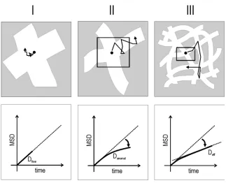
Influence of pores on diffusion: The influence of pores, or generally of geometrical constraints on the diffusional behaviour can be complex: (a) The diffusivity is in general reduced due to the presence of barriers, and it also depends on their geometrical shape and arrangement, for example, if the pores are straight, curved, interconnected or if they form bottleneck traps. (b) Particles interact with the walls of the pores, and may for example be subject to absorption/desorption kinetics.
Figure 15: Reduction of the diffusivity due to pores on different time scales.
trajectory or to the temporal and spatial resolution of the experimental apparatus, the diffusion will be perceived as unaffected by the geometrical constraint (case I in figure 15). If the temporal or spatial scale of the effects is comparable to the trajectory size the diffusivity becomes anomalous (case II in fig. 15). If the interactions take place on a very short time-scale, and if the molecules are otherwise free to diffuse in interconnected pores, the effects average out to give a normal diffusivity with a reduced effective
diffusion coefficient, Deff (case III in fig.15). The the ratio between the effective (case III) and the free (case I) diffusion coefficients (Dfree : Deff) can be expressed by a factor R, which comprises the influences of the geometry (e.g. the tortuosity) and interconnectivity of the pores (e.g. a 'labyrinth factor') for long observation times. The influence of the geometrical constraints can, however, be more complex, for example if the pores are so narrow that the molecules cannot pass each other (resulting in single-file diffusion). The effects of the geometrical constraints are difficult to predict analytically, and are usually compared with simulations.[Saxton97], [Regier05]
Distinguishing sub-populations: In the cases described so far the overall behaviour of one molecule or a group of molecules was assumed to be normally distributed. In a random walk, for example, the mean value for the individual mean squared displacements
〈r2(t)〉 corresponds to the most frequently found, or most probable value. The picture changes significantly if different sub-populations of diffusing molecules are present, or if one molecule changes its diffusional behaviour during its trajectory (e.g. by becomming trapped and released). In this case a more appropriate analysis of the diffusion is based on a population analysis, as explained in the following.
The individual mean square displacements 〈r2(t)〉 for every time lag t = nδt (defined as above) can be obtained by analysing the distribution p(u,t) of squared displacements (where r2 is substituted by u) for the relevant time lag:
p(u,t) =
− ) ( exp ) ( 1 2
2 r t
u t
p(u,t) is often given in the form of a histogram (figure 16a).
Figure 16: Conventional analysis of squared step distributions via histogrammes. a) An exemplary historgram (54 steps) showing the binned data and a fit according to eq. 11 for t=1 and b) histogram and fit for t=2 (53 steps).
A more elegant way to analyse diffusion, that avoids the necessity of artificially binning the data to obtain histograms is based on a statistical population analysis. The cumulative probability P(U,t), or the probability to find a squared step between 0 and U, is given by the integral betweeen 0 and U over p(u,t). The complementary function, C(U,t)gives the probability to find a squared step larger than U (see figure17a).
P(U,t) =
∫
p(u,t) du = 1 -U
0
−
) ( exp 2
t r
U
i
(12)
The complementary function (i.e. the probability to find a particle between 0 and infinity)
C(U,t) = 1 - P(U,t) (13)
Figure 17: Population analysis. a) Starting from the histogram it is possible to compute the cumulative probability P(U,t) and the complementary function C(U,t). b) P(U,t) and C(U,t) are plotted versus U. C(U,t) is plotted for two times t=1 and t=2.
C(U,t) is obtained from the experimental values of the individual squared displacements U, by sorting the values (longest squared step first) and assigning each a rank relative to the total number of steps j/N (N is the total number of steps).
The relative rank j/N of a specific squared displacement U gives the percentage of how many molecules have a smaller rank, or have a larger squared displacement - between U and infinity. This corresponds directly to C(U,t). This is shown in figure 18 for the same data set used to generate the histograms in figure 16. Note that the curve is visibly smoother, because it is not binned.
If a number (m) of sub-populations with different diffusion behavior are present, equation 11 becomes the sum of the individual distributions:
p(u,t) =
− = ( ) exp ) ( 1 2
1 2 r t
u t r A i m i i i
∑
(14)with relative amplitudes Ai (and the sum over all Ai being unity) The cumulative
probability is thus:
P(U,t) =
∫
p(u,t) du = 1 -U
0
∑
= − m i i i t r U A
1 2( )
exp (15)
The complementary function C(U,t) (i.e. equation 13), is for m sub-populations a sum of exponential decays with decay constants 〈r12(t)〉, 〈r22(t)〉, ... 〈rm2(t)〉. The ranked data can
then directly be fitted to a mono- bi-, tri- (and so on) exponential decay, which gives the respective decay constants for the m populations 〈r12(t)〉, 〈r22(t)〉, ... 〈rm2(t)〉.
The mean squared displacements obtained in this way can be evaluated against the time-lag t. For example, if different sub-populations are undergoing normal isotropic diffusion, with different diffusion coefficients, the respective diffusion coefficients Di are obtained
The same type of analysis can be used to characterize the distributions of step sizes for m different sub-populations (again, with the sum of the relative amplitudes Ai being unity).
The normalized distribution function of step lengths is:
q(r,t) =
( )
∑
= m i i i t r r A 1 2 2exp(-r2/〈ri2 (t)〉). (16)
The cumulative probability, or the probability to find a step with a length between 0 and R) distribution is thus
P(R,t) =
∫
q(r,t) dr = 1 -R
0
∑
= − m i i i t r R A 1 2 2 ) (
exp . (17)
The complementary function (the probability to find a setp larger than R)
C(R,t) = 1 - P(R,t) (18)
in the case of m sub-populations is a sum of m Gaussians centered at origin, with characteristic widths 〈r12(t)〉, 〈r22(t)〉, ... 〈rm2(t)〉. Again, the relative ranks of the
experimentally obtained step lengths correspond directly to C(R,t).
Using the described population analysis to determine the mean value (or mean values), has a series of advantages over other types of analysis that are based on making arbitrary cuts in the trajectory (for example around an area of reduced mobility that may appear to be particularly well-pronounced) or setting arbitrary binning and treshold values in the analysis of histograms. Firstly, there is no necessity to introduce these artificial
2.3.3. Methods in Comparison: The Measurement of Diffusion
A broad variety of methods can be used to study diffusion in porous materials. A brief overview and comparison is given in this section to put the experimentally obtained characterizations (via single molecule tracking) into a broader context.
Conventional, macroscopic approach: Methods based on the macroscopic approach evaluate the change of concentration in space with time c(x,t) using solutions to the Fickian equations (eqs 2,3). c(x,t) is monitored directly, for example via fluorescence (e.g. fluorescence recovery after photobleaching, FRAP, where the diffusion of a fluorescent dye into a photobleached area is observed), IR or NMR signals, as the concentration is directly proportional to the signal intensity. The major advantage of this approach lies in its simplicity and in the fact that it is not restricted to any particular type of molecule (e.g. fluorescent dyes). Limitations of this approach are: (a) The diffusion process has to be synchronized in some way for it to become observable. (b) The gained data does not contain the information availiable from the trajectories of the individual diffusing particles and depends on a series of assumptions.[Saxton97]
SMS / microscopic approach: The most straightforward method for the observation of diffusion is based on the direct observation of the individual diffusing particle (e.g. a fluorescent molecule). Diffusion parameters, such as the diffusion coefficient, the distribution of step sizes and angles between steps are obtained directly from the trajectory of the diffusing particle as described in the previous sub-sections. The major advantage of this method is that it allows to characterize diffusion in a very thorough way, because it does not discard the information contained in the individual trajectories for the analysis. It is possible to resolve different types of diffusional sub-populations and to visualize structural features in the trajectory directly (e.g. the appearance of fast or slow steps, or the presence of diffusional traps). This method is limited by the
(typically 10-9 or 10-10 M), and to slow diffusional processes (typically, with diffusion coefficients below 10-7 cm2s-1).
Another more indirect SMS method is based on the statistical analysis of the amount of particles, or molecules, diffusing in and out of a well-defined volume. This method is called fluorescence correlation spectroscopy (FCS). This approach determines the typical time a molecule stays in a given volume (eg. a confocal detection ellipsoid) by analysis of the autocorrelation function of intensity g(2)(τ) = 〈I(t)I(t+τ)〉〈I(t)〉-2. Typical concentrations of particles, or molecules for diffusion measurements are in the order of 10-8 M. The major advantage of this method is that it is capable of resolving very fast dynamic phenomena (diffusion, rotation, triplet blinking) taking place on a time scale of 0.1 µs. Very slow or rare processes however are not sensed by this method. Another limitation of this method is that the autocorrelation function has to be matched to a hypothetical
expression derived from a model of the diffusion process in order to obtain a parameter like the diffusion coefficient. Also, the spatial information contained in the individual trajectories is discarded by this technique.
Other methods: Among other methods that can be used to analyse diffusion are: Pulsed-field-gradient NMR, or PFG-NMR [Kukla96], quasi-elastic neutron scattering, or QENS [Benes01]. The strength of these methods lies in the possibility to probe the diffusional behaviour of any diffusing species, like water, methane and xenon, and are not restricted to the comparatively large fluorescent dye molecules.
'limited' to molecules with NMR-active nuclei and to a high concentrations of diffusing particles. The rule of thumb for 1H-PFG-NMR, for example is 1 proton per nm3. [Kärger, personal communication]. As an ensemble method PFG-NMR also fails to determine whether one molecule shows a heterogenous behaviour, or if a heterogeneity is caused by separate sub-populations of molecules coexisting in the same sample.
QENS probes the energy spectrum of neutrons which collide with the atoms of a diffusing species in a sample. If the collision is completely elastic, the energy of the scattered neutron will remain unaffected by the collision, unless the particle with which it collides is also moving due to translation, rotation or vibration (hence the term 'quasi'-elastic). These three movement components can be treated independently, since they occur on different time-scales.[Benes01] In the case of neutron collisions with diffusing molecules, additional components get added to and subtracted from the neutron's energy, causing the energy spectrum to broaden. The amount of broadening can be related to translational diffusion.[Benes01] The big disadvantage of QENS is that it is
experimentally very eleaborate (i.e. it requires a source of monochromatic neutrons), and that the final results are heavily dependent on the assumption of models.
Method Conc. [M] D [cm2s-1] Limited by: e.g. Ref.
PFG NMR > 10-12 < 10-4 Concentration [Kukla96] QENS > 10-12 < 10-4 Concentration [Benes01] FRAP > 10-13 < 10-4 Concentration [Saxton97] SMS-FCS 10-13 - 10-20 10-8 -10-4 Bleaching [Eggeling98] SMS-SPT 10-14 - 10-20 10-14-10-8 Frame Rate [Schmidt97]
The table above resumes the most important specifications for the described techniques. The concentration of diffusing particels is the limiting factor for all ensemble
measurements. The limiting factor for FCS is the photobleaching rate: Very slowly diffusing molecules would photobleach before they leave the irradiation area, leading to an artificially high diffusion coefficient. In SPT the limit is given by the speed with which an apparatus can record a sequence of images.
3. Experimental Setup and Background
The materials presented in the preceding chapter, the host-guest materials consisting of an organic dye molecule incorporated into the channels and voids of a molecular sieve are examined using fluorescence microscopy and SMS. In this chapter the experimental techniques used to acquire and to evaluate the data are discussed.
This chapter is subdivided into two sections: The first describes the used optical
3.1. Microscopy Techniques
Spatial Resolution in Microscopy: The idea behind microscopy is to obtain information from small regions in space. The central question for any type of microscopy is thus, how small such a region can be: The smaller the region, the better the spatial resolution
becomes. In optical microscopy, it can be shown that the spatial resolution is limited. The schematic illustration in figure 19 shows the necessary definitions and parameters that will be used in the following discussion.
Figure 19: Schematical picture illustrating the basic parameters and definitions used in the calculation of the spatial resolution of a microscopy apparatus.
A lens can neither focus light onto a point in space nor can it collect all the light coming from a point source in the focus. This is so, because it has a finite size and ultimately because of the existence of an angle of total reflection (α). This limited, effective size of a lens is characterized by a collection or focusation cone, described by the numerical aperture (NA) of the objective lens (see fig.19). The NA is defined as
NA = n1 · sin α, (19)
The main consequence of this limited size of the focusation cone is that the image of an object, projected onto the focal plane, will not contain the entire phase information needed to reconstruct the exact image of the object by interference. This loss of (phase-) information is finally what causes images to appear less sharp (see fig.20).
Figure 20: Influence of the nummerical apperture (NA) on the sharpness of an image. a) A lens with low NA produces blurred images. b) A lens with a higher NA collects a larger cone of light rays from the object (i.e. obtaining more phase infomation) and produces sharper images.
In effect a point-like object will appear as a diffraction pattern with a finite width. The intensity map of this pattern and its characteristic size can be used to characterize the resolution. This intensity map can be calulated for an idealized point-source for the different types of microscopy in dependence of the wavelength of the light in question (λ), of the NA and of the illumination and detection geometries. The resulting distribution function, IPSF(x,y,z) is called the point-spread function (PSF) of the optical apparatus. The PSF results from the convolution of the illumination and detection probabilities in space, Iill (x,y,z) and Idet(x,y,z).
Because of the cylindrical symmetry of most microscopy arrangements I(x,y,z) can
commonly be noted as I(r,z), where r is in an arbitrary direction parallel to the focal-plane of the microscope, and z is the optical axis.
The illumination and detection probabilities vary for different types of microscopy, resulting in different PSFs and in a series of advantages and limitations for the respective type of microscopy. The PSFs will be described in more detail below for the two
different fluorescence microscopy techniques used in this work: confocal microscopy and widefield imaging microscopy. Other types of optical microscopy are covered for
example in [Stelzer94], [Jung01] and [Seebacher02d]. Recent developments in fluorescence microscopy (e.g. using stimulated emission depletion) are covered in [Hell03] or [Hell04]; total internal reflection microscopy is covered in [Funatsu95] and [Ambrose99]; near field scanning optical microscopy is covered in [Hecht00] and [Dereux00].
3.1.1. Confocal Microscope
The basic idea behind confocal microscopy lies in the spatial superposition of the illumination and detection foci. As a consequence the illumination and the detection probabilities are nearly identical Iill(r,z) = Idet(r,z). Thus the intensity distribution of the PSF becomes:
IPSF(r,z) = Iill(r,z)2 (21)
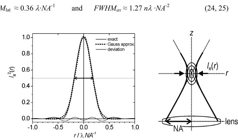
Iill(r,z)2 can be calculated. The exact result [Richards59], [Webb96], [Hell93] is difficult to handle mathematically. For most purposes, however, Iill(r,z) can conveniently be separated into a lateral Iill(r) and axial component Iill(z) and both components
approximated by simple Gaussians (in figure 21 this is shown for the lateral component):
In equations 22 and 23 the widths w depends on the used wavelength λ, on the NA and on the refractive index n1. They are empirically found to be wr= 0.15·λ·NA-1 for the lateral
component and wz = 0.54·nλ·NA-2 for the axial component. The full-width at half-maximum, FWHM, of these distribution functions are often used to characterize the resolution limit, or the minimal distance between two point-like objects, so that they still can be distinguished. The lateral FWHMlat and axial FWHMax are:
FWHMlat ≈ 0.36 λ·NA-1 and FWHMax≈ 1.27 nλ ·NA-2 (24, 25)
Figure 21: The exact intensity distribution function for the confocal PSF can be
approximated by a Gaussian. The FWHM can be used to characterize the resolution limit.
Experimentally, the focussed illumination is achieved by illuminating the specimen through the microscope objective with laser. The focussed detection is achieved by placing a spatial filter, a pinhole, in the detection pathway (as schematically illustrated in figure 22a). Note that strictly the factors 0.36 and 1.27 in equations 23 and 24 will also depend on the size of the pinhole pupil in detection. The given factors were obtained for the ideal case in which the pinhole corresponds exactly to the size of the focus.
discrepancy: (a) The pinhole is usually larger than the ideal size, (b) the optical elements (mirrors, lenses, etc.) are not perfect, (c) The refractive index between the object and the objective lens is typically inhomogenous. (d) The illumination beam is not perfectly collimated and not strictly monochromatic, and so is (e) the detection beam.
The ideal resolution volume element can be described by an ellipsoid with the diameters corresponding to the FWHMs given in equations 23 and 24. In figure 22b the size of the ellipsoid is depicted using λ=633 nm, NA=1.3 and n1=1.51 (immersion oil). The effective resolution ellipsoid (for the same conditions) is depicted in fig 22c. It was obtained experimentally, by acquiring a three-dimensional fluorescence pattern of a point-like emitter, for example an individual molecule - as it is considerably smaller than the wavelength in question.
Figure 22: Confocal microscopy. a) Illumination and detection geometry. b) The
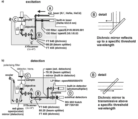
Experimental setup: The confocal microscope used in this work is based on a commercially availiable Zeiss model LSM 410, schematically depicted in fig. 23. A series of modifications were implemented on the LSM410, making it a versatile tool that can be used in single moelcule microscopy and spectroscopy. These will be explained in more detail below.
The specifications of the used lasers (A in fig. 23) are gathered in the following table:
Laser λex / nm Iex / µW (*)
HeCd 442 45
Kr+ 532 20000 Kr+ 568 20000
HeNe 594 3000
HeNe (int) 633 34
(*)maximum measured at objective barrel entrance (not attenuated)
All laser beams are collimated and directed to the scanning unit via a (suitable) dichroic mirror (B in fig. 23a). The laser beams are expanded and directed to the objective barrel to excite the sample (C in fig.23a). The maximum intensities of the used lasers given in the table above are measured at the entrance of the objective barrel. The typical excitation intensities for single molecule experiments lie between 1-50 µW.
The fluorescence of the sample (C in fig. 23b) is collected by the microscopy objective and is directed to the dichroic mirror (B in fig.23b). Red-shifted fluorescence light passes the dichroic mirror and is separated from unspecific or backscattered excitation light. The fluorecence light can then be routed to a series of detector units (D in fig. 23b).
xy-plane at a given depth z. The resulting two dimensional images are optical cross
sections of the sample at a specific depth z. (c) Finally, it is possible to gradually vary the depth z and make an xy-scan at different depths. In this way it is possible to reconstruct a three-dimensional image of the investigated specimen (cf. figure 24).
Figure 24: Image acquisition modes using the confocal microscope. (a) recording intensity from a fixed point in the sample. (b) xy-scans result in optical cross-sections (images) of the sample. (c) By varying the depth (z) a 3D image of the specimencan be reconstructed.
Temporal resolution: In case (a) - i.e. acquiring fluorescence from a specific point in the sample - the temporal resolution is limited only by the used detector and/or software. It can be as good as 100 ns, for example, using an autocorrelator device like the ALV-500. (b) The time resolution for the acquisition of a two-dimensional cross-section can be varied by adjusting the speed of the xy-scanner unit, which has an upper limit. For example, an image of 256 x 256 pixels cannot be recorded in less than 0.5 s with the LSM 410 hardware. (c) The time needed to record a stack of two-dimensional images is the product of the number of stacks multiplied with the time required to scan an
Detectors / Modifications: The built-in detector of the LSM410 (a photomultiplier tube) is not sensitive enough for the detection of the fluorescence from isolated molecules. An important modification in the detection arrangement is that the fluorescence signal can be routed to more sensitive external detectors, that possibilitate SMS.
Figure 25: Schematical arrangement of the external detectors.
The two external detectors used are: (a) An avalanche photodiode, APD, which is sensitive enough to detect the comparatively weak fluorescence signal of individual molecules, and (b) a prism-CCD spectrometer, which is also sensitive enough and can be used to record emission spectra of individual molecules.
APD: The most sensitive of the detectors used in this setup is the avalanche photodiode (EG&G SPCM-AQR-141). The APD produces a 9 ns TTL pulse upon detection of a photon (50 ns dead-time; 70% detection probability in the spectral region between 600 and 800 nm). The TTL pulses can be routed directly into an autocorrelator device (ALV-500) for the anaylsis of intensity fluctuations (with a temporal resolution of
approximately 100 ns), or processed by a pulse expander and re-routed to the microscope hardware to record images or intensity transients. The pulse expansion is required to convert the digital sequence of TTL pulses ('photon' / 'no photon') into a more gradual sum of pulses (≈ 'number of photons per time'), which can be processed appropriately by the microscope hard- and software. The pulse expander device also indicates the photon detection rate, and can be used to callibrate the intensity values indicated by the
CCD: Fluorescence light originating at the sample can be dispersed with an Amici-prism and detected with a peltier-cooled, back-illuminated CCD camera (Princeton Instruments, EEV 1300/100-EMB-chip) cf. schematical illustration in fig.26. The temporal resolution of the setup can be as good as 19 ms (with the system running instably), typically, however, sequences of spectra are obtained with a temporal resolution of 30-100 ms (depending on the fluorescence intensity). The time-limiting step for the aqcuisition of spectra is given by the chip read-out time. The spectral resolution of the setup in units per pixel varies with the dispersion strength of the prism, which in turn depends non-linearly on the respective wavelength of light The dispersion curve can be obtained empirically by imaging light with a known spectrum onto the CCD camera (cf. graphs in fig. 26). In effect, one pixel on the CCD covers between 0.5 and 2.5 nm of the spectrum in
wavelengths (from 450 to 700 nm, respectively). As will be seen in detail later the spectra can be callibrated and analysed automatically.
3.1.2. Widefield Imaging Microscope
Widefield microscopy stands conceptually in contrast to confocal microscopy. The difference results from the used illumination geometry, which in the widefield-imaging technique is more similar to that used in conventional microscopy. A laser (A in fig. 27) is used to exitate the sample. The beam is expanded and focussed onto the back-focal plane of the microscopy objective (B in fig. 27). On the sample side the beam is parallel and illuminates the sample uniformly (C and B detail in fig. 27).
Fluorescence is collected by the same objective. Residual exitation light is separated by using appropriate filters, in a similar way as shown before for confocal microscopy. The image, now originating simultaneously from the whole illuminated area is reconstructed on an area detector, such as a CCD camera (D in fig.26). The consequence for the PSF is that Iill (r,z) is merely a constant, because the sample is illuminated homogenously. Thus:
IPSF(r,z) = Idet(r,z) (26)
Idet(r,z) can be calculated and the exact result [Richards59], [Webb96], [Hell93], again, is difficult to handle mathematically. Idet(r,z) can however be separated into a lateral Idet(r) and axial component Idet(z) and both components approximated by simple Gaussians:
Idet(r) = I0 exp(-r2/ 2wr2) (27)
Idet(z) = I0exp (-z2/ 2wz2) (28)
with wr= 0.217·λ·NA-1 and wz = 0.72 nλ·NA-2 found empirically. The full-width at
half-maximum, FWHM, of eqns. 26 and 27 used to characterize the resolution limit are:
FWHMlat = 0.51 λ·NA-1 (29)
FWHMax = 1.7 nλ·NA-2 (30)
The sizes calculated for λ = 633 nm, n1 =1.51 (immersion oil) and NA =1.4 are, respectively for the lateral and axial FWHMs: 230 nm and 829 nm. The real sizes
Experimental setup / specifications: The setup is based on a Nikon Eclipse TE200 microscopy stand, using a 1.4 NA oil immersion objective (Plan Apochromat 100x) and a HeNe laser (633 nm 3mW power, NEC). The fluorescence images are recorded with an intensified multi-channel-plate-CCD (Pentamax / Princeton Instruments EEV, 512×512 pixel). Fluorescence light from the sample is projected onto the CCD on an area of approximately 150×150 pixels. The magnification factor, or the size of each pixel on the images can bedetermined from images of test patterns with a well-defined spacing. In all studies presented in this thesis the pixel size was 168 nm/pixel. Sequences of images can be acquired with a frame rate of 25 frames per second (or 40 ms per frame). An
exemplary sequence showing patterns from individual molecules is shown in figure 28.
Confocal and Widefield Microscopy in Comparison:
Confocal LSM 410 Widefield
lateral resolution (1.3 NA / 633 nm)
300 nm 300 nm
axial resolution 900 nm 3 µm
pol. measurements yes no (limited)
temp. res. 1D 0.1 µs -
temp. res. 2D 0.5 s (256 x 256) 20 ms (256 x 256)
temp. res. 3D 20 s -
address SM's yes no
installed wavelegths
442 nm 534 nm 568 nm 594 nm 633 nm
532 nm 633 nm
advantages (i) versatile, (ii) possibility to addresses individual molecules (iii) high depth resolution
(i) fast acquisition of 2D images (ii) parallel acquisition of SM signals
limitations (i) slow acquisition of images (ii) serial acquisition of SM data
3.2. Analysis Programs
The setup described in the previous sections produces an extensive amount of raw-data, in the form of (a) sequences of images (movies) showing the diffusion of individual particles, (b) sequences of spectra showing diverse forms of spectral dynamics from an individual emitter, (c) sequences of polarization dependent intensity traces that
characterize the orientation of individual emitters and (d) sequences of intensity transients which can be used to characterize the photostability of a certain type of molecule. In the evaluation of this data every sub-set of data (every frame in a movie, every spectrum in a sequence of spectra, etc.) has to be analysed individually, for example callibrated or fitted. It is not feasible to evaluate this amount of data manually. Suitable programs that analyze this kind of data automatically are, however, not commercially availiable.
In the next sub-sections four different sets of programmes are presented, which have been conceived and written in order to evaluate the different types of data automatically. The first set of programmes are utilized in the tracking of individual diffusing particles in a sequence of microscopy images. The second set of programmes are used in the analysis of spectral parameters. The third set is used to evaluate polarization dependent data to determine the orientational angles of individual molecules. The last set of programmes was written in order to obtain photostability parameters of the used dye molecules such as a number of emitted photons prior to photobleaching and typical on and off-times.
3.2.1. Evaluation of Diffusion

![Figure 6: Typical examples for zeolite structures. From [ZeoliteAtlas05]](https://thumb-us.123doks.com/thumbv2/123dok_us/8204288.1370453/23.612.180.434.319.543/figure-typical-examples-zeolite-structures-zeoliteatlas.webp)