An Algorithm for the Simulation of the Magnetized
Neutron Star Cooling
H. Grigorian1,2,a, A. Ayriyan1, E. Chubarian2, A. Piloyan3, and M. Rafayelyan4
1Joint Institute for Nuclear Research, Joliot-Curie 6, 141980 Dubna, Moscow Region, Russia
2Yerevan State University, Alek Manyukyan 1, 0025 Yerevan, Republic of Armenia
3Yerevan Physics Institute, A. Alikhanian Brothers 2, 0036 Yerevan, Republic of Armenia
4University of Bordeaux, 351 Cours de la Libération, F-33400 Talence, France
Abstract. A model and algorithm for the cooling of the magnetized neutron stars are presented. The cooling evolution described by a system of parabolic partial differential equations with non-linear coefficients is solved using the Alternating Direction Implicit method. A difference scheme and the preliminary results of simulations are presented.
1 Introduction
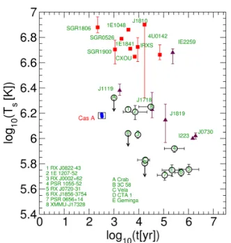
Figure 1: Observational data of age and tem-perature of compact stars. Squares – AXPs and SGRs neutron stars with magnetic field from 1014G up to 1015G. Triangles – radio-quiet stars with field around 1013G. Circles – radio-pulsars with field≤1012G.
Modelling of magnetized neutron stars cooling process is an interesting subject for the investi-gations of the internal structure of such objects. The main aspect is the investigation of the nu-clear matter properties at extremely high densi-ties. The magnetic field of compact object when
it is more than 1014 G has a significant influence
on the heat transport inside the star and can give observational effects on the surface temperatures. The model of cooling evolution is given by a sys-tem of parabolic partial differential equations with
non-linear temperature depending thermal coeffi
-cients and cooling (via neutrinos) and heating (due to magnet field decay) sources.
Due to the axial symmetry of the field and spherical symmetry of the matter distribution in-side, the problem can be described using spheri-cal coordinates in spatial 2D. For the solution we choose the Alternating Direction Implicit (ADI)
method [1, 2]. In the difference scheme we use
non-constant spatial steps and self-correcting time
ae-mail: [email protected]
C
step. We investigate the special boundary conditions in the center and on the surface of the star con-figuration. At the current stage of the study we are going to present some preliminary results of the
cooling simulations to demonstrate the efficiency of our 2D cooling algorithm.
The nowadays observational data of the magnetized neutron star (Fig. 1, for the table of data with corresponding references, see [3]) could not be explained by 1D cooling simulations neglecting the magnetic field inside. The inclusion of the magnetic field is necessary but not sufficient yet [3, 4]. In this work we focus on an algorithm of 2D simulation of the cooling of a magnetized neutron star.
2 Equations for Thermal Evolution of the Magnetized Compact Star
The neutron star is surrounded by a gravitational field which, in the approximation of slow rotation of the stars, can be described by the metric tensor of the space-time manifold [5]
ds2=−e2Φdt2+e2Λdr2+r2dΩ2. (1)
The compact star configuration is constructed with the use of the equation of state (EoS) of the stellar matter based on the knowledge of the nuclear matter [6]. The coefficients of the metric tensor as well as characteristics of the matter distribution are self-consistent solutions of the Einstein equation (specially for this case TOV [5, 6]) where the temperature effect on the internal structure could be neglected because of the high density inside the star.
On the other hand the thermal evolution of the star can be described using the energy balance equation, which has parabolic form:
cveΦ∂∂T
t +∇ · (e
2ΦF) =e2ΦQ, (2)
wherecvis the specific heat per unit volume andQis the energy loss/gain by neutrino emission, Joule heating, accretion heating, etc. The vectorFcorresponds to the heat flux.
The thermal properties of the stellar matter are investigated under of different nuclear matter cool-ing scenarios [7–11].
The flux is created due to the temperature gradient and tends to equilibrate the temperature
F = −e−Φκˆ·∇(eΦT).
Here ˆκis the thermal conductivity, which is a tensor under an enough strong magnetic field of the star. Hereafter we will use the notations ˜T ≡eΦT and ˜F ≡e2ΦF. The flux components (in spherical coordinates) of the dipole magnetic field are:
˜
Fr=−eΦ
κrre−Λ∂rT˜+κrθ r ∂θT˜
, F˜θ=−eΦκθ
re−Λ∂rT˜+κθθ
r ∂θT˜
,
with theφ-component vanishing identically due to the axial symmetry.
The magnetic field, which affects the conductivity, leads to anisotropy along and orthogonal to
the field. The relation between the conductivity components is defined in terms of the magnetization parameterωBτ:
κ
κ⊥ =1+(ωBτ)
2, (3)
whereτis the particle relaxation time [12], andωB is the classical gyrofrequency corresponding to
the magnetic field strengthB,
ωB= eB
mis the effective mass,eis the charge of the particle in the magnetic field, andcis the speed of light. Using the unit vectorbof the magnetic dipole the flux, we get:
F=−eΦκ⊥
∇T˜+(ωBτ)2b·∇T˜·b+ωBτb×∇T˜. (5)
When the magnetic field is parallel to the axiszone hasb=(cosθ,−sinθ,0). So for the compo-nents of the conductivity we get:
κrr = 1+(ωBτ)2ξ2
1+(ωBτ)2 κ,
κθr = κrθ=ξ
1−ξ2(κ −κ⊥),
κθθ = 1+(ωBτ)
2(1−ξ2)
1+(ωBτ)2 κ.
For simplicity we will use the following notations:ξ≡cos(θ), ˜Q≡e2ΦQ.
The introduction of the new variableξand of the accumulated massm=4π ρr2dr(hereρis the
energy density of the matter) instead ofθandrtransforms the thermal evolution equation (2) to the following form
∂u
∂t =D1
∂ ∂m
B1m∂∂u
m+B1ξ
∂u
∂ξ
+D2∂ξ∂
B2m∂∂u
m+B2ξ
∂u
∂ξ
+QB.
The sought-for function isu=log( ˜T) and the coefficients are
B1m≡4πr4ρe−Λ(1+(ωBτ)ξ2)k⊥T e˜ Φ, B2m≡4πrρe−Λξ
1−ξ2ωBτ)2k⊥T e˜ Φ,
B1ξ≡rξ
1−ξ2(ωBτ)2k⊥T e˜ Φ, B2ξ≡
1+(ωBτ)21−ξ2 1−ξ2k
⊥T e˜ Φ/r2,
andD1≡4πD2ρe−Λ,D2≡(cvT)−1,QB≡D2Q˜.
3 2D Scheme for Mixed Implicit and Explicit Methods
Numerical calculations were done using the most convenient ADI method [1, 2] from the point of
view of the stability. The discretization with respect tomwas done taking into account the energy
distributionρ(r). This function is the solution of a single compact star for a given central density or a given total mass. At each given distancerjfrom the center, we have the grid pointsmj. The mass at a givenjis the same for all angles, thereforeξcould be considered as an independent coordinate.
The steps of discretization aremj±1/2 =±
mj±1−mj
andmj=(1/2)
Δmj+1/2+ Δmj−1/2
=
(1/2)mj+1−mj−1
. Similar notations are used for the angleξas well as for any function F(r, θ):
Fi,j±1/2=(1/2)
Fi,j±1+Fi,j
.
The first order partial derivatives have been approximate by first order finite differences,
∂u
∂m
i,j±1/2
=±ui,j±1−ui j
mj±1/2 ,
∂u
∂ξ
i±1/2,j
=±ui±1ξi,j−ui j
±1/2 .
For the second order derivatives, theRandS operators corresponding to a same or to mixed variables were defined,
R(1)ui j≡ −D1∂∂ m
B1m∂∂u
m
i,j
=−D1i,j mj
B1m,i,j+1/2
ui,j+1−ui,j
mj+1/2 −B1m,i,j−1/2
ui j−ui j−1
mj−1/2
R(2)ui j ≡ −D2
∂ ∂ξ B2ξ
∂u
∂ξ i,j=−
D2i,j
ξi B2ξ,i+1/2,,jui+
1,j−ui,j
ξi+1/2 −B2ξi−1/2,j
ui j−ui−1,j ξi−1/2 ,
and
S(1)ui j=D1∂∂ m
B1ξ∂∂ξu
i j
= D1i,j
2mj
B1ξ,i,j+1
ui+1,j+1−ui−1,j+1
2ξi −B1ξ,i,j−1
ui+1j−1−ui−1,j−1
2ξi
,
S(2)ui j=D2
∂ ∂ξ
B2m∂∂u
m
i,j
= D2i,j
2ξi
B2m,i+1,jui+
1,j+1−ui+1,j−1
2mj −B2m,i−1,j
ui−1j+1−ui−1,j−1
2mj
.
After discretization of the time with the stepsΔtn, the differential equation of the problem can be written as:
un+1−un tn
+σR(1)un+1+(σ−1)R(2)un+1=(σ−1)R(1)un−σR(2)un+S(1)un+S(2)un+QB.
The introduced parameterσstands for the ADI method: atσ=1 the implicit method is used with
respect tom, while atσ=0, with respect toξ.
The non-vanishing elements in the right hand side of this algebraic equation can be written in the following form
X[i][j] = σK (1)
i,j+1/2
Δmj
2 +(σ−1)K
(2)
i+1/2,j (Δξi)2 ,
Z[i][j] = σK (1)
i,j−1/2
Δmj
2 +(σ−1)K
(2)
i−1/2,j
(Δξi)2 , (6)
Y[i][j] = 1/tn−X[i][j]−Z[i][j],
S[i][j] = un
i j/tn+(σ−1)
R(1)un
i j−σ
R(2)un
i j+
S(1)un
i j+
S(2)un
i j+[QB]i j,
where we use the following notations: X[i][j] andZ[i][j]are upper and lower diagonal vectors
corre-spondingly,Y[i][j]is the main diagonal vector. For solving the obtained tri-diagonal algebraic system,
the Thomas algorithm is used [13, 14].
Figure 2: Relation between the mantle tem-peratureTmand the surface temperatureTs
In (6), the Ki(1),j andKi(2),j are the centred mean values
Ki(1),j±1/2=D1i,jB1mi,j±1/2 Δmj
Δmj±1/2,
K(2)i±1/2,j=D2i,jB2ξi±1/2,j
Δξj
Δξj±1/2.
To complete the tri-diagonal algebraic system, a set of boundary conditions obeying to the phys-ical requirements, at the center and on the sur-face of the neutron star is defined as follows [15]. All fluxes of heat from all directions have to vanish at the center. This leads toX[i][0] =0. Therefore,
At the surface we assume that the flux of the energy along the radial direction has to equate the flux of energy of the photon emission:
Lm(i,J)=2πR2σT˜s4(i)Δξi,
where J is the maximal value of the index j, σ is the Boltzmann constant andTs is the surface
temperature, which is connected toTm, the mantle temperature under the core (Fig. 2):
ui,J=log ˜Tm(i).
A detailed discussion of this point was reported in [7].
From symmetry reasons, the tangential fluxes on the polar and equatorial planes also are zero
Lξ(i=0,j)=Lξ(i=I,j)=0:
Lξ(i,j)=
B1ξ∂∂ξu
i,j
=B1ξ,i,j
ui+1,j−ui−1,j
2Δξi .
4 Some Features of the Simulations and Conclusions
To demonstrate the work of our algorithm we provide simulations with model coefficients, which
are taking into the account the main features of the physical properties of the thermal coefficients.
Particularly, we use the cooling mechanism of the neutrino emission, the so called modified URCA process (see for details [16]). We also vary the magnetic field, however we don’t include the Joule heating from the decay of magnetic field.
As it can be seen from the Fig. 3a, due to absence of additional anisotropic heating sources, the temperature distribution in all directions becomes isotropic after 50 years of evolution. And we can notice as well that this property is independent of the value of the initial anisotropic distribution of the temperature.
One can notice that, if the temperature along some direction is initially smaller then the temper-ature at the beginning of the isotropic era it heats up during the evolution (see dotted lines for the lowest arrow in Fig. 3a). It means that the heat conducting process dominates the neutrino cooling.
We notice that a period of 50−100 years is short enough to be able to compare this results with
observations, because all available data (Fig. 1) are for objects older than at least 500 years. On the other hand one can see that the temperature values at the beginning of the isotropic era are around the same what are the observational temperatures of already cold magnetars.
It means that the heat retention inside the star for such a long time could not be just the effect of the anisotropy due to the magnetization. It is even hard to argue that the observed temperatures of red point in Fig. 1 are estimated only for small area around the poles of the stars.
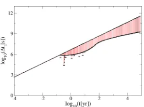
In the Fig. 3b we demonstrate the automatic choice of the time-step of the numerical algorithm. The top line on this figure is the predicted time-step, the bottom curve is the modified time-step to provide stability of the algorithm. The automatic choice of the time-step is needed mainly due to the non-trivial mass distribution inside the star.
Acknowledgements
(a) Surface temperature evolution of neutron star with massm= 1.4sun. Each color corresponds to cooling curves for different azimuthal angles of one object.
(b) The choice of the time-step during the numerical simulation.
Figure 3: Simulation results of the coolings of magnetars
References
[1] A. Samarskii and P. Vabishchevich, Computational Heat Transfer, Volume 1 (John Wiley &
Sons Ltd., Chichester, England, 1995)
[2] N. Yanenko,Fractional step methods for solution of multidimensional problems of mathematical
physics(Nauka, Moscow, 1967) (in russian)
[3] D. Aguilera, J. Pons, and J. Miralles, The Astroph. J. Lett.673, 2, L167–L170 (2008) [4] D.N. Aguilera, J.A. Pons, and J.A. Miralles, Astron. & Astroph.486, 255–271 (2008)
[5] C. Misner, K. Thorne, and J. Wheeler,Gravitation(W.H. Freeman and Co., San Francisco, 1973)
[6] F. Weber,Pulsars as Astrophysical Laboratories for Nuclear and Particle Physics(IOP
Publish-ing, Bristol, Great Britain, 1999)
[7] D. Blaschke, H. Grigorian, and D.N. Voskresensky, Astron. & Astroph.424, 979–992 (2004) [8] H. Grigorian and D.N. Voskresensky, Astron. & Astroph.444, 3, 913–929 (2005)
[9] H. Grigorian, D. Blaschke, and D. Voskresensky, Phys. Rev. C71, 045801 (2005)
[10] D. Page, J. Lattimer, M. Prakash, and A. Steiner, The Astroph. J. Suppl. Ser.155, 623 (2004) [11] D. Page, J. Lattimer, M. Prakash, and A. Steiner, The Astroph. J.707, 2 (2009)
[12] V. Urpin and D. Yakovlev, Soviet Astronomy24, 425 (1980)
[13] L. Thomas,Elliptic Problems in Linear Differential Equations over a Network(Watson Sci.
Comput. Lab Report, Columbia University, New York, 1949)
[14] W. Press, S. Teukolsky, W. Vetterling, and B. Flannery,Numerical Recipes, third ed.(Cambridge
University Press, New York, 2007)
[15] D. Yakovlev, K. Levenfish, A. Potekhin, O. Gnedin, and G. Chabrier, Astron. & Astroph.417,
169–179 (2004)