Analysis of the Spatial Distribution of Galaxies
by Multiscale Methods
J-L. Starck
DAPNIA/SEDI-SAP, Service d’Astrophysique, CEA-Saclay, 91191 Gif-sur-Yvette, France Email:[email protected]
V. J. Mart´ınez
Observatori Astron`omic de la Universitat de Val`encia, Edifici d’Instituts de Paterna, Apartat de Correus 22085, 46071 Val`encia, Spain
Email:[email protected]
D. L. Donoho
Department of Statistics, Stanford University, Sequoia Hall, Stanford, CA 94305, USA Email:[email protected]
O. Levi
Department of Statistics, Stanford University, Sequoia Hall, Stanford, CA 94305, USA Email:[email protected]
P. Querre
DAPNIA/SEDI-SAP, Service d’Astrophysique, CEA-Saclay, 91191 Gif-sur-Yvette, France Email:[email protected]
E. Saar
Department of Cosmology, Tartu Observatory, Toravere 61602, Estonia Email:[email protected]
Received 17 June 2004; Revised 17 February 2005
Galaxies are arranged in interconnected walls and filaments forming a cosmic web encompassing huge, nearly empty, regions between the structures. Many statistical methods have been proposed in the past in order to describe the galaxy distribution and discriminate the different cosmological models. We present in this paper multiscale geometric transforms sensitive to clusters, sheets, and walls: the 3D isotropic undecimated wavelet transform, the 3D ridgelet transform, and the 3D beamlet transform. We show that statistical properties of transform coefficients measure in a coherent and statistically reliable way, the degree of clustering, filamentarity, sheetedness, and voidedness of a data set.
Keywords and phrases:galaxy distribution, large-scale structures, wavelet, ridgelet, beamlet, multiscale methods.
1. INTRODUCTION
Galaxies are not uniformly distributed throughout the uni-verse. Voids, filaments, clusters, and walls of galaxies can be observed, and their distribution constrains our cosmologi-cal theories. Therefore we need reliable statisticosmologi-cal methods to compare the observed galaxy distribution with theoretical models and cosmological simulations.
The standard approach for testing models is to define a point process which can be characterized by statistical
descriptors. This could be the distribution of galaxies of a specific type in deep redshift surveys of galaxies (or of clus-ters of galaxies).1 In order to compare models of structure formation, the different distribution of dark matter particles
1Making 3D maps of galaxies requires knowing how far away each galaxy
in N-body simulations could be analyzed as well, with the same statistics.
The two-point correlation functionξ(r) has been the pri-mary tool for quantifying large-scale cosmic structure [1]. Assuming that the galaxy distribution in the Universe is a realization of a stationary and isotropic random process, the two-point correlation function can be defined from the probability δP of finding an object within a volume ele-ment δV at distancer from a randomly chosen object or position inside the volume: δP = n(1 +ξ(r))δV, where n is the mean density of objects. The function ξ(r) mea-sures the clustering properties of objects in a given vol-ume. It is zero for a uniform random distribution, pos-itive (resp., negative) for a more (resp., less) clustered distribution. For a hierarchical clustering or fractal pro-cess, 1 +ξ(r) follows a power-law behavior with exponent D2 −3. Since ξ(r) ∼ r−γ for the observed galaxy dis-tribution, the correlation dimension for the range where ξ(r) 1 is D2 3 − γ. The Fourier transform of the correlation function is the power spectrum. The di-rect measurement of the power spectrum from redshift sur-veys is of major interest because model predictions are made in terms of the power spectral density. It seems clear that the real space power spectrum departs from a sin-gle power-law ruling out simple unbounded fractal mod-els [2]. The two-point correlation function can been gen-eralized to the N-point correlation function [3, 4], and all the hierarchy can be related with the physics responsi-ble for the clustering of matter. Nevertheless they are diffi -cult to measure, and therefore other related statistical mea-sures have been introduced as a complement in the sta-tistical description of the spatial distribution of galaxies [5], such as the void probability function [6], the mul-tifractal approach [7], the minimal spanning tree [8, 9, 10], the Minkowski functionals [11, 12], or the J func-tion [13, 14] which is defined as the ratio J(r) = (1− G(r))/(1−F(r)), where F is the distribution function of the distance r of an arbitrary point in R3 to the near-est object in the catalog, and G is the distribution func-tion of the distance r of an object to the nearest ob-ject. Wavelets have also been used for analyzing the pro-jected 2D or the 3D galaxy distribution [15, 16, 17, 18, 19].
New geometric multiscale methods have recently emerged, the beamlet transform [20, 21] and the ridgelet transform [22]; these allow us to represent data containing, respectively, filaments and sheets, while wavelets represent well isotropic features (i.e., clusters in 3D). As each of these three transforms is tuned to a specific kind of feature, all of them are useful and should be combined to describe a given catalog.
Sections2,3, and4describe, respectively, the 3D wavelet transform, the 3D ridgelet transform, and the 3D beam-let transform. It is shown in Section 5through a set of ex-periments how these three 3D transforms can be combined in order to describe statistically the distribution of galax-ies.
2. THE 3D WAVELET TRANSFORM
2.1. The undecimated isotropic wavelet transform
For eacha >0,b1,b2,b3∈R3, thewaveletis defined by
ψa,b1,b2,b3:R3−→R,
ψa,b1,b2,b3
x1,x2,x3
=a−3/2·ψ
x1−b1 a ,
x2−b2 a ,
x3−b3 a
. (1)
Given a function f ∈L2(R3), we define its wavelet coef-ficients by
Wf :R4−→R,
Wf
a,b1,b2,b3
=
ψa,b1,b2,b3(x)f(x)dx.
(2)
Figure 1shows an example of 3D wavelet function. It is standard to digitize the transform for datac(x,y,z) withx,y,z ∈ {1,. . .,N}as follows. The wavelet transform of a signal produces, at each scale j, a set of zero-mean coef-ficient values {wj}. Letφ be a lowpass filter and we define φj(x) = φ(2jx) and cj = c∗φj. Using an undecimated isotropic wavelet decomposition [23], the set{wj}has the same number of pixels as the signal and this wavelet trans-form is redundant. Furthermore, using a wavelet defined as the difference between the scaling functions of two successive scales
1 8ψ
x 2,
y 2,
z 2
=φ(x,y,z)−1 8φ
x 2,
y 2,
z 2
, (3)
the original cubec=c0can be expressed as the sum of all the wavelet scales and the smoothed arraycJ:
c0,x,y,z=cJ,x,y,z+ J
j=1
wj,x,y,z. (4)
The setw= {w1,w2,. . .,wJ,cJ}represents the wavelet trans-form of the data. If we letW denote the wavelet transform operator and N the pixels in c, the wavelet transform w (w = Wc) has (J+ 1)N pixels, for a redundancy factor of J+ 1. The scaling functionφis generally chosen as a spline of degree 3, and the 3D implementation is based on three 1D sets of (separable) convolutions. Like the scaling functionφ, the wavelet functionψ is isotropic (seeFigure 2). More de-tails can be found in [23,24].
3. THE 3D RIDGELET TRANSFORM
3.1. The 2D ridgelet transform
−10−5 0 5 10 −0.5
0 0.5 1
−10−5 0 5 10 −10
−5
0 5 10
60 50 40 30 20 10 60
50 40
30 20
10 0
y
0 10 20
30 40 50 60
x
−10−5 0 5 10 −0.5
0 0.5 1
−10−5 0 5 10 −10
−5
0 5 10
Figure1: Example of wavelet function.
θ1
x1
x2
θ1line
(a)
θ1
θ2
x1
x2
x3
(θ1,θ2) line
(b)
Figure2: Definition of angle1θ1andθ2in (a)R2(2D case) and (b)R3(3D case).
Select a smooth functionψ ∈L2(R), satisfying
admissi-bilitycondition
ˆ ψ(ξ)2
|ξ| dξ <∞, (5)
which holds ifψhas a sufficient decay and a vanishing mean
ψ(t)dt=0 (ψcan be normalized so that it has unit energy 1/(2π)|ψˆ(ξ)|2dξ = 1). For eacha > 0,b ∈ R, andθ
1 ∈ [0, 2π[, we define theridgeletby
ψa,b,θ1:R2−→R,
ψa,b,θ1
x1,x2
=a−1/2·ψ
x1cosθ1+x2sinθ1−b
a
. (6)
Given a function f ∈ L2(R2), we define its ridgelet coeffi -cients by
Rf :R3−→R,
Rf
a,b,θ1
=
ψa,b,θ1(x)f(x)dx.
(7)
(a)
−2 0 2
−0.2 0 0.2 0.4 0.6 0.8 1
(b)
Figure3: Example of 2D ridgelet function.
60 50 40 30 20 10 60
50 40
30 20
10 0
y
0 10 20
30 40 50 60
x
−2 −1
0 1
2
−0.2 0 0.2 0.4
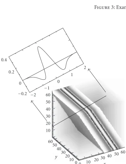
Figure4: Example of ridgelet function.
Figure 3(left) shows an example ridgelet function. This function is constant along lines x1cosθ+x2sinθ = const. Transverse to these ridges it is a wavelet (seeFigure 3(b)).
3.2. From 2D to 3D
The 3D continuous ridgelet transform of a function f ∈ L2(R3) is given by
Rf :R4−→R,
Rf
a,b,θ1,θ2
=
ψa,b,θ1,θ2(x)f(x)dx,
(8)
(1)3D-FFT. Compute ˆc(k1,k2,k3), the 3D FFT of the cube
c(i1,i2,i3).
(2)Cartesian-to-spherical conversion. Using an interpolation scheme, substitute the sampled values of ˆcobtained on the Cartesian coordinate system (k1,k2,k3) with sampled values in a spherical coordinate system (θ1,θ2,ρ). (3)Extract lines. Extract the 3N2lines (of sizeN) passing
through the origin and the boundary of ˆc.
(4)1D-IFFT. Compute the 1D inverse FFT on each line. (5)1D-WT. Compute the 1D wavelet transform on each
line.
Algorithm1: The 3D ridgelet transform algorithm.
where a > 0,b ∈ R,θ1 ∈ [0, 2π[, and θ2 ∈ [0,π[. The ridgelet function is defined by
ψa,b,θ1,θ2:R3−→R,
ψa,b,θ1,θ2
x1,x2,x3
=a−1/2·ψ
x1cosθ1cosθ2+x2sinθ1cosθ2+x3sinθ2−b
a
.
(9)
Figure 4shows an example of ridgelet function. It is a wavelet function in the direction defined by the line (θ1,θ2), and it is constant along the orthogonal plane to this line.
As in the 2D case, the 3D ridgelet transform can be built by extracting lines in the Fourier domain. Letc(i1,i2,i3) be a cube of size (N,N,N); the steps can be seen inAlgorithm 1 steps.
Figure 5shows the 3D ridgelet transform flowgraph. The 3D ridgelet transform allows us to detect sheets in a cube.
Local 3D ridgelet transform
x1
x2
x3
Euclidian space
kx1
kx2
kx3
Fourier space
θ1
θ2
(θ1, θ2) line
Plane⊥(θ1, θ2) line
Spatial radiusρ ρ
Lines (θ1, θ2) line
Plane⊥(θ1, θ2) line,
scalej
1D WT
Lines 1D wavelet transform
of (θ1, θ2) line
Scale 1 Scalej
Scalej+1
Radon transform 1D wavelet transform
Figure5: 3D ridgelet transform flowgraph.
introduced [26]. The cubecis decomposed into blocks of lower side-lengthbso that for aN×N×Ncube, we count N/bblocks in each direction. After the block partitioning, the tranform is tuned for sheets of sizeb×band of thicknessaj, aj corresponding to the different dyadic scales used in the transformation.
4. THE 3D BEAMLET TRANSFORM
4.1. Definition
The X-ray transform of a continuum function f(x,y,z) with (x,y,z)∈R3is defined by
(X f)(L)=
Lf(p)dp, (10)
whereLis a line inR3, andpis a variable indexing points in the line. The transformation contains all line integrals of f. The beamlet transform (BT) can be seen as a multiscale digi-tal X-ray transform. It is multiscale transform because, in ad-dition to the multiorientation and multilocation line integral calculation, it integrated also over line segments at different lengths. The 3D BT is an extension to the 2D BT, proposed by Donoho and Huo [20].
The system of 3D beams
The transform requires an expressive set of line segments, including line segments with various lengths, locations, and orientations lying inside a 3D volume.
A seemingly natural candidate for the set of line segments is the family ofallline segments between each voxel corner and every other voxel corner, the set of3D beams. For a 3D data set withn3voxels, there areO(n6) 3D beams. It is infeasi-ble to use the collection of 3D beams as a basic data structure
since any algorithm based on this set will have a complexity with lower bound ofn6and hence be unworkable for typical 3D data size.
4.2. The beamlet system
A dyadic cubeC(k1,k2,k3,j)⊂[0, 1]3is the collection of 3D points
x1,x2,x3
:
k1 2j,
k1+ 1
2j
×
k2 2j,
(k2+ 1) 2j
×
k3 2j,
k3+ 1
2j
,
(11)
where 0≤k1,k2,k3<2jfor an integerj≥0, called the scale. Such cubes can be viewed as descended from the unit cubeC(0, 0, 0, 0) =[0, 1]3by recursive partitioning. Hence, the result of splittingC(0, 0, 0, 0) in half along each axis is the eight cubesC(k1,k2,k3, 1) whereki ∈ {0, 1}(seeFigure 6), splitting those in half along each axis we get the 64 subcubes C(k1,k2,k3, 2) whereki ∈ {0, 1, 2, 3}, and if we decompose the unit cube inton3voxels using a uniformn-by-n-by-ngrid withn=2Jdyadic, then the individual voxels are then3cells C(k1,k2,k3,J), 0≤k1,k2,k3< n.
0 0.5 1
1 0.5
0 0 0.5 1
C(0,0,0,0)
(a)
0 0.5 1
1 0.5
0 0 0.5 1
C(1,1,1,1)
C(0,1,1,1)
C(0,1,0,1)
C(1,0,1,1)
C(1,0,0,1)
C(0,1,0,1) (b)
Figure6: Dyadic cubes.
(a) (b)
Figure7: Examples of beamlets at two different scales: (a) scale 0 (coarsest scale) and (b) scale 1 (next finer scale).
dyadic cube at scale jhas a side-length of 2J−jvoxels, we get O(24(J−j)) beamlets associated with the dyadic cube and a to-tal ofO(24J−j)=O(n4/2j) beamlets at scalej. If we sum the number of beamlets at all scales we getO(n4) beamlets.
This gives a multiscale arrangement of line segments in 3D with controlled cardinality ofO(n4), the scale of a beam-let is defined as the scale of the dyadic cube it belongs to so lower scales correspond to longer line segments and finer scales correspond to shorter line segments.Figure 7shows 2 beamlets at different scales.
To index the beamlets in a given dyadic cube, we use slope-intercept coordinates. For a data cube ofn×n×n vox-els, consider a coordinate system with the cube center of mass at the origin and a unit length for a voxel. Hence, for (x,y,z) in the data cube we have|x|,|y|,|z| ≤n/2. We can consider three kinds of lines:x-driven,y-driven, andz-driven, depend-ing on which axis provides the shallowest slopes. Anx-driven line takes the form
z=szx+tz, y=syx+ty (12)
with slopes sz,sy, and interceptstz andty. Here the slopes |sz|,|sy| ≤ 1. y- andz-driven lines are defined with an in-terchange of roles betweenxandyorz, as the case may be.
The slopes and intercepts run through equispaced sets:
sx,sy,sz∈
2
n : = − n 2,. . .,
n 2−1
,
tx,ty,tz∈
:−n 2,. . .,
n 2−1
.
(13)
Beamlets in a data cube of sidenhave lengths between n/2 and√3n(the main diagonal).
Computational aspects
60 50 40 30 20 10 60
50 40
30 20
10 0
y
0 10 20
30 40 50 60
x
−10−5 0 5 10 −0.5
0 0.5 1
−10−5 0 5 10 −10
−5 0 5 10
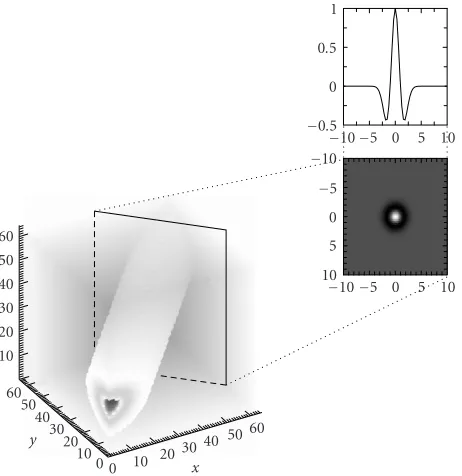
Figure8: Example of beamlet function.
We will mention that in many cases there is no interest in the coarsest scales coefficient that consumes most of the compu-tation time and in that case the overall running time can be significantly faster. The algorithms can also be easily imple-mented on a parallel machine of a computer cluster using a system such as MPI in order to solve bigger problems.
(1)3D-FFT. Compute ˆc(k1,k2,k3), the three-dimensional FFT of the cubec(i1,i2,i3).
(2)Cartesian to spherical conversion. Using an interpolation scheme, substitute the sampled values of ˆcobtained on the Cartesian coordinate system (k1,k2,k3) with sampled values in a spherical coordinate system (θ1,θ2,ρ). (3)Extract planes. Extract the 3N2planes (of sizeN×N)
passing through the origin (each line used in the 3D ridgelet transform defines a set of orthogonal planes; we take the one including the origin).
(4)2D-IFFT. Compute the 2D inverse FFT on each plane. (5)2D-WT. Compute the 2D wavelet transform on each
plane.
Algorithm2: The 3D beamlet transform algorithm.
4.3. The FFT-based transformation
Letψ ∈L2(R2) be a smooth function satisfying a 2D vari-ant of theadmissibilitycondition, the 3D continuous beamlet transform of a function f ∈L2(R3) is given by
Bf :R5−→R,
Bf
a,b1,b2,θ1,θ2
=
ψa,b,θ1,θ2(x)f(x)dx,
(14)
wherea >0,b1,b2 ∈R,θ1 ∈[0, 2π[, andθ2 ∈[0,π[. The beamlet function is defined by
ψa,b1,b2,θ1,θ2:R3−→R,
ψa,b1,b2,θ1,θ2
x1,x2,x3
=a−1/2·ψ
−x1sinθ1+x2cosθ1+b1
a ,
x1cosθ1cosθ2+x2sinθ1cosθ2−x3sinθ2+b2
a
. (15)
Figure 8shows an example of beamlet function. It is con-stant along lines of direction (θ1,θ2), and a 2D wavelet func-tion along plane orthogonal to this direcfunc-tion.
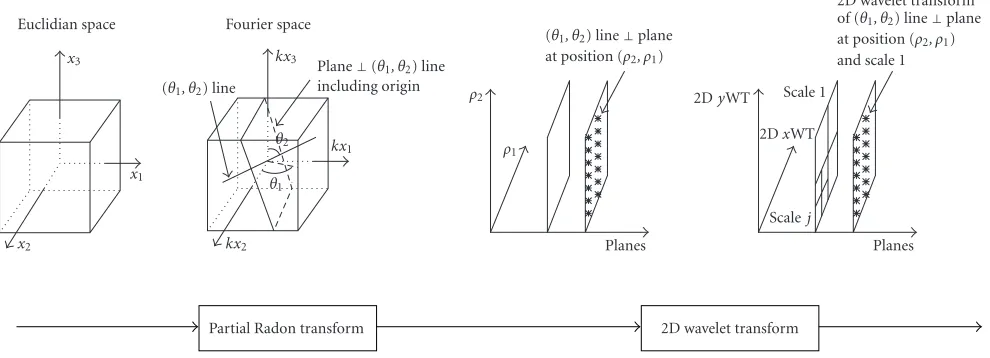
The 3D beamlet transform can be built using the “gen-eralized projection-slice theorem” [27]. Let f(x) be a func-tion onRn; and letRadmf denote them-dimensional par-tial Radon transform along the firstm directions,m < n.
Radmf is a function of (p,µm;xm+1,. . .,xn),µm a unit di-rectional vector in Rn (note that for a given projection an-gle, them-dimensional partial Radon transform of f(x) has (n−m) untransformated spatial dimensions and a (n−m +1)-dimensional projection profile). In addition, let {F f}(k) denote then-dimensional Fourier transform wherexandk are conjugate variables.
The Fourier transform of the m-dimensional partial radon transformRadmf is related to the Fourier transform of f (F f) by the projection-slice relation
Fn−m+1Radmf
k,km+1,. . .,kn
= {F f}kµm,km+1,. . .,kn. (16)
x1
x2
x3
Euclidian space
kx1
kx2
kx3
Fourier space
θ1
θ2
(θ1, θ2) line
Plane⊥(θ1, θ2) line
including origin
(θ1, θ2) line⊥plane
at position (ρ2, ρ1)
ρ2
ρ1
Planes
2D wavelet transform of (θ1, θ2) line⊥plane
at position (ρ2, ρ1)
and scale 1 2DyWT
2DxWT
Planes Scale 1
Scalej
Partial Radon transform 2D wavelet transform
Figure9: 3D beamlet transform flowgraph.
5. EXPERIMENTS
5.1. Experiment 1
We have simulated three data sets containing, respectively, a cluster, a plane, and a line. To each data set, Poisson noise has been added with eight different background levels. We applied the three transforms on the 24 simulated data sets. The coefficient distribution from each transformation was normalized using twenty realizations of a Poisson noise hav-ing the same number of counts as in the data.
Figure 10 shows the maximum value of the normal-ized distribution versus the noise level for our three simu-lated data sets. As expected, wavelets, ridgelets, and beam-lets are, respectively, the best for detecting clusters, sheets, and lines. A feature can typically be detected with a very high signal-to-noise ratio in a matched transform, while re-maining indetectible in some other transforms. For exam-ple, the wall is detected at more than 60σ by the ridgelet transform, but at less than 5σ by the wavelet transform. The line is detected almost at 10σ by the beamlet trans-form, and with worse than 3σ detection level by wavelets. These results show the importance of using several trans-forms for an optimal detection of all features contained in a data set.
5.2. Experiment 2
We use here two simulated data sets to illustrate the discrim-inative power of multiscale methods. The first one is a sim-ulation from stochastic geometry. It is based on a Voronoi model. The second one is a mock catalog of the galaxy distri-bution drawn from aΛ-CDM N-body cosmological model [29]. Both processes have very similar two-point correlation functions at small scales, although they look quite different and have been generated following completely different al-gorithms.
(i) The first comes from Voronoi simulation. We locate a
point in each of the vertices of a Voronoi tessellation of 1500 cells defined by 1500 nuclei distributed follow-ing a binomial process. There are 10 085 vertices lyfollow-ing within a box of 141.4h−1Mpc side.
(ii) The second point pattern represents the galaxy po-sitions extracted from a cosmological Λ-CDM N-body simulation. The simulation has been carried out by the Virgo consortium and related groups (see http://www.mpa-garching.mpg.de/Virgo). The simu-lation is a low-density (Ω =0.3) model with cosmo-logical constantΛ = 0.7. It is, therefore, an approxi-mation to the real galaxy distribution [29]. There are 15 445 galaxies within a box with side 141.3h−1Mpc. Galaxies in this catalog have stellar masses exceeding 2×10¹⁰M
.
Figure 11 shows the two simulated data sets, and Figure 12 shows the two-point correlation function curve for the two-point processes. The two-point fields are diff er-ent, but as can be seen inFigure 12, both have very similar two-point correlation functions in a huge range of scales (2 decades).
Wavelet Ridgelet Beamlet
0.01 0.1 1
Noise level
N
o
rm
aliz
ed
maxim
u
m
value
1 1.5 2 2.5 3
0 5 10 15 20 25 30 0 5 10 15 20 25 30
0 5 10 15 20 2530
(a)
Wavelet Ridgelet Beamlet
N
o
rm
aliz
ed
maxim
u
m
value
0.01 0.1 1
Noise level 10
20 30 40 50 60
0 5 10 15 20 25 30 0 5 10 15 20 25 30
0 5 10 15 20 2530
(b)
Wavelet Ridgelet Beamlet
N
o
rm
aliz
ed
maxim
u
m
value
0.01 0.1 1
Noise level 2
4 6 8
0 5 10 15 20 25 30 0 5 10 15 20 25 30
0 5 10 15 20 2530
(c)
20 40 60 80 100 120 140
20 40 60 80 100 120 140
20 40 60
80 100120 140 (a)
20 40 60 80 100 120 140
20 40 60 80 100 120 140
20 40 60
80 100120 140 (b)
(c) (d)
Figure 11: Simulated data sets. (a) The Voronoi vertices point pattern and (b) the galaxies of the GIF Λ-CDM N-body simulation. (c) One 10h−1width slice of each data set.
Voronoi
Λ-CDM (GIF)
0.01 0.1 1 10
r
0.1 1 10 100 1000 10 000 100 000
ξ
(
r
)
Figure12: The two-point correlation function of the Voronoi ver-tices process and the GIFΛ-CDM N-body simulation. They are very similar in the range [0.02, 2]h−1Mpc.
5.3. Experiment 3
In this experiment, we have used aΛ-CDM simulation based on the N-body hydrodynamical code, RAMSES [30]. The simulation uses an adaptive mesh refinement (AMR) tech-nique, with a tree-based data structure allowing recursive grid refinements on a cell-by-cell basis. The simulated data were obtained using 2563particles and 4.1×10⁷cells in the AMR grid, reaching a formal resolution of 81923. The box size was set to 100h−1Mpc, with the following cosmological parameters:
Ωm=0.3, Ωλ=0.7, Ωb=0.039,
h=0.7, σ8=0.92.
(17)
We used the results of this simulation at six different redshifts (z = 5, 3, 2, 1, 0.5, 0). Figure 14 shows a projec-tion of the simulated cubes along one axis. We applied the 3D wavelet transform, the 3D beamlet transform, and the 3D ridgelet transform on the six data sets. Letσ2
W,z,j,σR2,z,j, σ2
Simulated file 1 Simulated file 2
0 1.5 3 4.6
Ridgelet 0 0.5 1 1.5 2 2.5 3
Wa
ve
le
t
0 1.4 2.9 4.3
Beamlet
(a)
Simulated file 1 Simulated file 2
0 1.9 3.8 5.7
Ridgelet 0 1 2 3 4 5 6
Wa
ve
le
t
0 1.8 3.6 5.5
Beamlet
(b)
Simulated file 1 Simulated file 2
0 2.1 4.3 6.4
Ridgelet 0 5 10 15
Wa
ve
le
t
0 5.8 11.7 17.5
Beamlet
(c)
Simulated file 1 Simulated file 2
0 3.6 7.2 10.8
Ridgelet 0 5 10 15 20 25
Wa
ve
le
t
0 6.3 12.6 18.8
Beamlet
(d)
Figure13: Skewness and kurtosis for the two simulated data sets: (a) skewness, scale 1, (b) skewness, scale 2, (c) kurtosis, scale 1, and (d) kurtosis, scale 2.
Figure 15, shows, respectively, from top to bottom, the wavelet spectrum Pw(z,j) = σW2,z,j, the beamlet spectrum Pb(z,j) = σ2
B,z,j, and the ridgelet spectrum Pr(z,j) = σ2
R,z,j. In order to see the evolution of matter distribution with redshift and scale, we calculate the ratioMw/b(j,z) = Pw(z,j)/Pb(z,j) andMw/r(j,z)=Pw(z,j)/Pr(z,j).
Figure 16shows theMw/bandMw/rcurves as a function ofzandFigure 17shows theMw/b−1 andMw/r−1 curves as a func-tion of the scale number j.
Figure14:Λ-CDM simulation at different redshifts.
6. CONCLUSION
We have introduced in this paper a new method to analyze catalogs of galaxies based on the distribution of coefficients obtained by several geometric multiscale transforms.
We have introduced two new multiscale decompositions, the 3D ridgelet transform and the 3D beamlet transform, matched to sheetlike and filament features, respectively. We described fast implementations using FFTs. We showed that combining the information related to wavelet, ridgelet, and beamlet coefficients leads to a new description of point cat-alogs. In this paper, we described transform coefficients us-ing skewness and kurtosis, but another recent statistic esti-mator such the higher criticism[31] could be used as well. Each multiscale transform is very sensitive to one kind of fea-ture: wavelets to clusters; beamlets to filaments; and ridgelets to walls. A similar method has been proposed for analyz-ing CMB maps [32] where both the curvelet and the wavelet transforms were used for the detection and the discrimina-tion of non-Gaussianities. This combined multiscale statistic is very powerful and we have shown that two data sets with identical two-point correlation functions are clearly distin-guished by our approach. These new tools lead to better con-straints on cosmological models.
z=5
z=3
z=2
z=1
z=0.5
z=0
0 2 4
Scale number 2.2×10⁻¹
1×10²
4.6×10⁴
2.2×10⁷
Lo
g
(r
at
io)
(a)
z=5
z=3
z=2
z=1
z=0.5
z=0
0 1 2
Scale number 10−2
100
102
104
Lo
g
(r
at
io)
(b)
z=5
z=3
z=2
z=1
z=0.5
z=0
0 1 2
Scale number 10−1
101
103
105
Lo
g
(r
at
io)
(c)
Scale 3 Scale 2 Scale 1
5 4 3 2 1 0
z
1 2 3 4
Ratio
(a)
Scale 3 Scale 2 Scale 1
5 4 3 2 1 0
z
0.133 0.4 0.667 0.933
Ratio
(b)
Figure16: (a) Wavelet/beamletMw/b(z,j) and (b) wavelet/ridgelet
Mw/r(z,j) curves for the scale numberjequal to 1,2, and 3.
ACKNOWLEDGMENTS
We wish to thank Romain Teyssier for giving us the Λ -CDM simulated data used in the third experiment. This work has been supported by the Spanish MCyT project AYA2003-08739-C02-01 (including FEDER), the Generalitat Valen-ciana project GRUPOS03/170, the National Science Founda-tion Grant DMS-01-40587 (FRG), and the Estonian Science Foundation Grant 4695.
REFERENCES
[1] P. J. E. Peebles, The Large-Scale Structure of the Universe, Princeton University Press, Princeton, NJ, USA, 1980. [2] M. Tegmark, M. R. Blanton, M. A. Strauss, et al., “The
three-dimensional power spectrum of galaxies from the sloan digital
z=5
z=3
z=2
z=1
z=0.5
z=0
0 1 2
Scale number 0.25
0.4 0.63 1
Lo
g
(r
at
io)
(a)
z=5
z=3
z=2
z=1
z=0.5
z=0
0 1 2
Scale number 1.58
2.51 3.98 6.31
Lo
g
(r
at
io)
(b)
Figure 17: (a) Beamlet/wavelet 1/Mw/b(z,j) and (b) ridgelet/ wavelet 1/Mw/r(z,j) curves at different redshifts.
sky survey,”The Astrophysical Journal, vol. 606, no. 2, part 1, pp. 702–740, 2004.
[3] S. Szapudi and A. S. Szalay, “A new class of estimators for the N-point correlations,”Astrophysical Journal Letters, vol. 494, no. 1, pp. L41–L44, 1998.
[4] P. J. E. Peebles, “The galaxy and mass N-point correlation functions: a blast from the past,” inHistorical Development of Modern Cosmology, V. J. Mart´ınez, V. Trimble, and M. J. Pons-Border´ıa, Eds., vol. 252 ofASP Conference Series, Astronomi-cal Society of the Pacific, San Francisco, Calif, USA, 2001. [5] V. J. Mart´ınez and E. Saar,Statistics of the Galaxy Distribution,
Chapman & Hall/CRC press, Boca Raton, Fla, USA, 2002. [6] S. Maurogordato and M. Lachieze-Rey, “Void probabilities
[7] V. J. Mart´ınez, B. J. T. Jones, R. Dom´ınguez-Tenreiro, and R. van de Weygaert, “Clustering paradigms and multifractal measures,”The Astrophysical Journal, vol. 357, no. 1, pp. 50– 61, 1990.
[8] S. P. Bhavsar and R. J. Splinter, “The superiority of the min-imal spanning tree in percolation analyses of cosmological data sets,”Monthly Notices of the Royal Astronomical Society, vol. 282, no. 4, pp. 1461–1466, 1996.
[9] L. G. Krzewina and W. C. Saslaw, “Minimal spanning tree statistics for the analysis of large-scale structure,”Monthly No-tices of the Royal Astronomical Society, vol. 278, no. 3, pp. 869– 876, 1996.
[10] A. G. Doroshkevich, D. L. Tucker, R. Fong, V. Turchaninov, and H. Lin, “Large-scale galaxy distribution in the Las Cam-panas Redshift Survey,”Monthly Notices of the Royal Astro-nomical Society, vol. 322, no. 2, pp. 369–388, 2001.
[11] K. R. Mecke, T. Buchert, and H. Wagner, “Robust morpho-logical measures for large-scale structure in the universe,” As-tronomy & Astrophysics, vol. 288, no. 3, pp. 697–704, 1994. [12] M. Kerscher, “Statistical analysis of large-scale structure in the
universe,” inStatistical Physics and Spatial Statistics: The Art of Analyzing and Modeling Spatial Structures and Pattern Forma-tion, K. Mecke and D. Stoyan, Eds., vol. 554 ofLecture Notes in Physics, pp. 36–71, Springer, Berlin, Germany, 2000. [13] M. N. M. Van Lieshout and A. J. Baddeley, “A
nonparamet-ric measure of spatial interaction in point patterns,”Statistica Neerlandica, vol. 50, no. 3, pp. 344–361, 1996.
[14] M. Kerscher, M. J. Pons-Border´ıa, J. Schmalzing, et al., “A global descriptor of spatial pattern interaction in the galaxy distribution,”The Astrophysical Journal, vol. 513, no. 2, part 1, pp. 543–548, 1999.
[15] E. Escalera, E. Slezak, and A. Mazure, “New evidence for subclustering in the Coma cluster using the wavelet analy-sis,”Astronomy & Astrophysics, vol. 264, no. 2, pp. 379–384, 1992.
[16] E. Slezak, V. de Lapparent, and A. Bijaoui, “Objective detec-tion of voids and high-density structures in the first CfA red-shift survey slice,”The Astrophysical Journal, vol. 409, no. 2, pp. 517–529, 1993.
[17] V. J. Mart´ınez, S. Paredes, and E. Saar, “Wavelet analysis of the multifractal character of the galaxy distribution,”Monthly No-tices of the Royal Astronomical Society, vol. 260, no. 2, pp. 365– 375, 1993.
[18] A. Pagliaro, V. Antonuccio-Delogu, U. Becciani, and M. Gam-bera, “Substructure recovery by three-dimensional discrete wavelet transforms,”Monthly Notices of the Royal Astronom-ical Society, vol. 310, no. 3, pp. 835–841, 1999.
[19] T. Kurokawa, M. Morikawa, and H. Mouri, “Scaling analysis of galaxy distribution in the Las Campanas Redshift Survey data,”Astronomy & Astrophysics, vol. 370, no. 2, pp. 358–364, 2001.
[20] D. L. Donoho and X. Huo, “Beamlets and multiscale image analysis,” inMultiscale and Multiresolution Methods, vol. 20 of
Lecture Notes in Computational Science and Engineering, pp. 149–196, Springer, New York, NY, USA, 2001.
[21] D. L. Donoho and O. Levi, “Fast x-ray and beamlet trans-forms for three-dimensional data,” inModern Signal Process-ing, D. Rockmore and D. Healy, Eds., vol. 46 ofMathematical Science Research Institute Publications, Cambridge University Press, Cambridge, UK, March 2002.
[22] E. J. Cand`es and D. L. Donoho, “Ridgelets: the key to high dimensional intermittency?”Philosophical Transactions of the Royal Society of London A, vol. 357, pp. 2495–2509, September 1999.
[23] J.-L. Starck, F. Murtagh, and A. Bijaoui,Image Processing and
Data Analysis: The Multiscale Approach, Cambridge Univer-sity Press, Cambridge, UK, 1998.
[24] J.-L. Starck and F. Murtagh, “Astronomical Image and Data Analysis,” @#pages, Springer, Berlin, Germany, 2002. [25] J.-L. Starck, E. J. Cand`es, and D. L. Donoho, “The curvelet
transform for image denoising,”IEEE Trans. Image Processing, vol. 11, no. 6, pp. 670–684, 2002.
[26] E. J. Cand`es, “Harmonic analysis of neural networks,”Applied and Computational Harmonic Analysis, vol. 6, no. 2, pp. 197– 218, 1999.
[27] P. C. Lauterbur and Z.-O. Liang,Principle of Magnetic Reso-nance Imaging, IEEE Press, New York, NY, USA, 2000. [28] D. L. Donoho, O. Levi, J.-L. Starck, and V. J. Mart´ınez,
“Multi-scale geometric analysis for 3D catalogs,” inAstronomical Data Analysis II, J.-L. Starck and F. Murtagh, Eds., vol. 4847 of Pro-ceedings of SPIE, pp. 101–111, Waikoloa, Hawaii, USA, August 2002.
[29] G. Kauffmann, J. M. Colberg, A. Diaferio, and S. D. M. White, “Clustering of galaxies in a hierarchical universe—I. Methods and results atz=0,”Monthly Notices of the Royal Astronomical Society, vol. 303, no. 1, pp. 188–206, 1999.
[30] R. Teyssier, “Cosmological hydrodynamics with adaptive mesh refinement—A new high resolution code called RAM-SES,”Astronomy & Astrophysics, vol. 385, no. 1, pp. 337–364, 2002.
[31] D. L. Donoho and J. Jin, “Higher criticism for detecting sparse heterogeneous mixtures,” Tech. Rep., Statistics Department, Stanford University, Stanford, Calif, USA, 2002.
[32] J.-L. Starck, N. Aghanim, and O. Forni, “Detection and discrimination of cosmological non-Gaussian signatures by multi-scale methods,” Astronomy & Astrophysics, vol. 416, no. 1, pp. 9–17, 2004.
J-L. Starck has a Ph.D. degree from the University Nice-Sophia Antipolis and a Ha-bilitation degree from the University Paris XI. He was a Visitor at the European Southern Observatory (ESO) in 1993, at UCLA in 2004, and at the Statistics De-partment, Stanford University, in 2000 and 2005. He has been a researcher at the service d’Astrophysique, CEA-sacloy, since 1994. His research interests include image
pro-cessing, statistical methods in astrophysics, and cosmology. He is also author of two books entitledImage Processing and Data Analy-sis: the Multiscale Approach, andAstronomical Image and Data Anal-ysis.
V. J. Mart´ınezreceived his Ph.D. degree in mathematics from the University of Valen-cia in 1989, after preparing his thesis at NORDITA, Copenhagen, where his Adviser was Bernard Jones. In 1991, he got a perma-nent position at the University of Valencia as an Associate Professor in astronomy and astrophysics. He is currently the Director of the Observatori Astron ´omic dela Universi-tat de Valencia. He works on the sUniversi-tatistical
D. L. Donohois Anne T. and Robert M. Bass Professor in the hu-manities and sciences at Stanford University. He received his A.B. degree in statistics at Princeton University where his thesis Adviser was John W. Tukey and his Ph.D. degree in statistics at Harvard University, where his thesis adviser was Peter J. Huber. He is a Mem-ber of the US National Academy of Sciences and of the American Academy of Arts and Sciences.
O. Levi is a faculty member in the De-partment of Industrial Engineering and Management, Ben-Gurion University of the Negev, Beer Sheva, Israel. He received the B.S. degree in mathematics and industrial engineering and the M.S. degree in in-dustrial engineering from Ben-Gurion Uni-versity, Israel. He earned his Ph.D. degree in scientific computing and computational mathematics from Stanford University in
2004. His thesis title was entitled “Multiscale geometric analysis of 3-D data sets” and he worked under the supervision of Professor D. Donoho. His fields of interest include scientific computing, matrix computation, discrete Fourier analysis, and MSG algorithms.
P. Querrehas an Engineering degree from the Institut National Polytechnique de Toulouse. He has been working for the last five years at the Service d’Astrophysique, Saclay, on image and signal processing ap-plications. He got involved in the develop-ment of new methods of 2D and 3D redun-dant multiscale transforms. His main re-search interests are signal and image pro-cessing algorithms.
E. Saarreceived his Cand. Sci. (Ph.D.) de-gree in theoretical physics at Tartu Univer-sity in 1971, and his Dr. Astr. degree at the same university in 1991. He has worked all his life at Tartu Observatory, at positions ranging from a Programmer to a Vice Di-rector. Currently he is the Head of the Cos-mology Department. He has written papers on general relativity (inhomogeneous cos-mologies), physics of galaxies (spiral