A reduced-complexity scheme using message passing for location tracking

R E S E A R C H

Open Access

A reduced-complexity scheme using message

passing for location tracking

Yih-Shyh Chiou

1

, Fuan Tsai

1*

, Chin-Liang Wang

2

and Chin-Tseng Huang

3

Abstract

This article presents a low-complexity and high-accuracy algorithm using message-passing approach to reduce the computational load of the traditional tracking algorithm for location estimation. In the proposed tracking scheme, a state space model for the location-estimation problem can be divided into many mutual-interaction local

constraints based on the inherent message-passing features of factor graphs. During each iteration cycle, the message with reliability information is passed efficiently with an adaptive weighted technique and the error propagation law, and then the message-passing approach based on prediction-correction recursion is to simplify the implementation of the Bayesian filtering approach for location-estimation and tracking systems. As compared with a traditional tracking scheme based on Kalman filtering (KF) algorithms derived from Bayesian dynamic model, the analytic result and the numerical simulations show that the proposed forward and one-step backward tracking approach not only can achieve an accurate location very close to the traditional KF tracking scheme, but also has a lower computational complexity.

Keywords:Bayesian approach, data reliability, factor graphs, location tracking, one-step backward, wireless communication

1. Introduction

With the rapid advance in technologies and infrastruc-tures, wireless communication systems have been getting great momentum due to the convenience that they can provide. Among the various applications in the systems, location-based services (LBSs) are appearing in our daily life both indoors and outdoors [1]. In other words, various LBSs have been set up in companies, universities, stations, airports, shopping malls, and even households; they are becoming more and more popular, and they are conse-quently attracting high attentions in industry and acade-mia to investigate their characteristics in every aspect. However, providing customers with tailored LBSs is a fun-damental problem [2,3], and the positioning and tracking mobile terminals (MTs) are considered a key problem in wireless environments. Therefore, the location accuracy and computational complexity are two major challenges in location-estimation systems. Furthermore, for integrating the use of information and communications technology

and the use of telecommunications and informatics (tele-matics) in wireless networks, good location information can help optimize resource allocation and improve coop-eration. In other words, accurate positioning and tracking schemes are essential for useful location-estimation sys-tems [4-6], and accurate locations can be improved with location tracking algorithms.

The fundamental phases of tracking systems are based on the prediction (time update) and the correction (measurement update) [7]; the role of location tracking algorithms is to perform recursive state estimation, which is given by state equation and observation equa-tions. For location-estimation techniques using tracking algorithms, Kalman filtering (KF) algorithms are consid-ered optimal for the linear Gaussian model, and they have been introduced to enhance the accurate estima-tion of the locaestima-tion-estimaestima-tion system [7-20]. Neverthe-less, the high accurate location based on the traditional KF algorithm requires high computational complexity, and direct implementation of the KF equations may be too complex to be applied to practical systems [21]. To improve location-estimation efficiency, it would be use-ful to develop an algorithm with high location accuracy

* Correspondence: [email protected]

1

Center for Space and Remote Sensing Research, National Central University, Jhongli 32001, Taiwan

Full list of author information is available at the end of the article

and low computational complexity. Consequently, some fixed coefficient or degenerate form algorithms were proposed to avoid repeatedly calculating the Kalman gain, and the computational load of these schemes is lower than the traditional KF algorithm [7,17,22-25]. However, these schemes are only suitable for tracking the MT in steady-state environments; the coefficients of these algorithms have to be extracted again when these algorithms change its coefficients for different situations. Therefore, to reduce the computational load of the KF tracking algorithm and to get more flexible tracking schemes than some fixed coefficient or degenerate form algorithms are worth developing low-complexity techni-ques for location-estimation and tracking systems. For these reasons, some location-estimation algorithms are based on factor graphs (FGs) [26-30], the errors of these algorithm are expressed in the form of a Gaussian prob-ability density function (PDF). In addition, with compu-tationally attractive technique, location tracking schemes based on a state space model can be derived from the Bayesian dynamic model [31-33], which is a probabilistic framework for state estimation using the Markov assumption. Namely, to effectively simplify the imple-mentation of Bayesian approach, the message of tracking scheme can be represented by the statistical properties of the estimated variables. In other words, for a linear dynamic system, these approaches can be applied for location-estimation systems, and then a location track-ing algorithm based on message-passtrack-ing propagation can efficiently be cycled between the prediction and cor-rection phases.

In this article, an efficient location tracking scheme based on an adaptive weighted technique with low com-putational load and good location accuracy is proposed to estimate an MT’s location. Specifically, instead of using the traditional KF tracking scheme, the FG with the distributed feature makes the decomposition of the joint distribution to be functions of the variables. There-fore, a forward approach for location estimation and one-step backward approach for speed estimation are pro-posed to simplify the implementation for the location-estimation system. The analytic and simulation results demonstrate that the proposed forward and one-step backward (FOSB) tracking scheme passing the reliable messages between the prediction and correction phases can achieve an accurate location very close to that of the KF tracking scheme. In addition, the computational load of the proposed scheme is lower than the traditional KF algorithm, and the proposed tracking scheme can easily be implemented.

The remainder of this article is organized as follows. Section 2 presents the background on inference for loca-tion-estimation techniques. Section 3 applies the proposed

FOSB tracking scheme to overcome the computational complexity of the traditional tracking scheme. Perfor-mance evaluation and simulation results are discussed in Section 4. Finally, the conclusion is given in Section 5.

2. Background

2.1. Preliminary

For the system and the measurement of the MT at time k, let us consider the dynamic system described in state space form. The mathematical models based on prob-ability densities can be taken as [31]

State equation :xk+1=funx(xk,uk)↔f(xk+1|xk) (1)

Observation equation:zk=funz(xk,vk)↔h(zk|xk), (2) wherexk, funx(·), and uk are the state vector,

transi-tion functransi-tion, and process noise with known distribu-tion, respectively;zk,funz(·), and vkare the observation

vector, observation function, and observation noise with known distribution, respectively. f(xk+ 1|xk) and h(zk|

xk) are the transition PDF and observation PDF,

respec-tively. By these equations, the hidden states xkdisturbed

byukand the datazkdisturbed byvkare assumed to be

generated by functionsfunx(·), and funz(·), respectively.

We assume that the initial statex0 is distributed accord-ing to a density function f(x0), and that h(z0|x0) is the distribution of the initial observation. In addition, the Bayesian approach assumes that the dynamic system is Markovian, and all relevant information is contained in the current-state variable. As a result, the joint probabil-ity densprobabil-ity of states and observations based on the prob-ability chain rule can be expressed as

p(x0:K,z0:K) =f(x0)h(z0|x0)

K

k=1

f(xk|xk−1)h(zk|xk),(3)

wherex0:k≜(x0, ...,xk) andz0:k≜(z0, ...,zk). The

solu-tion of the sequential estimasolu-tion problem is obtained by the algorithm sequentially estimating the states of a sys-tem as a set of observations becomes available. In fact, both directed and undirected graphs allow a global func-tion of several variables to be expressed as a product of factors over subsets of those variables [34]. According to the concept of directed graphs, with Bayesian networks for expressing causal relationships between random vari-ables, a graphical representation of (3) between states and observations can be illustrated in Figure 1 [31].

In addition, for the Bayesian approach at time k, assume thatp(xk|z0:k) is known, and the objective is to

find p(xk+1|z0:k+1). According to the Markov structure

Prediction step (time update)

p(xk+1|z0:k) =

p(xk|z0:k)f(xk+1|xk)dxk. (4)

Correction step (measurement update)

p(xk+1|z0:k+1) =

h(zk+1|xk+1)p(xk+1|z0:k) p(zk+1|z0:k)

, (5)

wherep(zk+1|z0:k) is the predictive distribution ofzk+1 given the past observationsz0:k. The prediction-correction

recursion relations in (4) and (5) form the sequential scheme for the Bayesian approach.

2.2. State and measurement models

In this article, the useful notation of the tracking algorithm can be taken as follows. The value of vectorx(t) at a dis-crete time instantt=tkis denoted byxk. A best estimate

ofx(t) at timet=tkgiven the observations up to timet=

tjis denoted by a double-subscript notation withxk|j. Moreover, for location tracking, there are three useful cases denoted as follows: the one-step fixed-lag smoothing is xk|k+1=xk whenk<j=k+ 1: the best estimation is xk|k=xˆk when k = j; the best one-step prediction is xk+1|k=x˜k+1 whenk+1 >j=k. Therefore, for the linear

Gaussian model, the mathematical models of the linear dynamic system and of the measurement can be denoted as a state space model by

State equation

xk+1=kxk+uk,uk∼N(0,Qk) (6)

E{unuTk}=

Qkforn=k

0 forn=k =δ(k−n)Qk Observation equation

zk=Hkxk+vk, vk∼N(0,Rk) (7)

E{vnvTk}=

Rkforn=k

0 forn=k =δ(k−n)Rk,

wherexk,Fk,uk, andQkare the state matrix, state

tran-sition matrix, model noise matrix, and model noise covar-iance matrix, respectively;zk,Hk,vk, andRkare the actual

measurement matrix, measurement transition matrix, measurement noise matrix, and measurement noise covar-iance matrix, respectively;ukandvkare zero-mean

inde-pendent Gaussian vectors with covariance matricesQk

andRk, respectively. According to the prediction and

cor-rection steps in (4) and (5), the mathematical equations and phases of the KF algorithm derived from Bayesian dynamic model are described in Appendix 1.

2.3. Operations of prediction-correction recursion

According to the inherent distributed feature of the FG and the distributive law of multiplications to make the decomposition of the joint distribution to be functions of the variables [34], the messages of the reliable infor-mation can be processed and passed among variable nodes and factor nodes. The fundamental concepts about the works of FG algorithm with message-passing structure are illustrated in Appendix 2. Therefore, the useful operations of prediction-correction recursion based on message passing are introduced as follows. 2.3.1. The correction phase (measurement update)

Assume that each message is a Gaussian PDF, with the notation as

N(x;m,σ2)∝exp(−(x−m) 2

2σ2 ). (8)

The product of any KGaussian PDF is also Gaussian and is expressed as [26,34]

K

k=1

N(x;mk,σk2)∝N(x;mˆ,σˆ2), (9)

1

(

1

|

)

k

f

k k

x

x

x

x

k2

f

(

x

k2

|

x

k1

)

1

(

|

)

k

f

k k

x

x x

z

_k-1

z

_k

z

_k+1

z

_k+2

x

_k-1

x

_k

x

_k+1

x

_k+2

1

(

1

|

1

)

k

h

k k

z

z

x

z

k

h

( |

z x

k k

)

z

k1

h

(

z

k1

|

x

k1

)

z

k2

h

(

z

k2

|

x

k2

)

1

(

1

|

2

)

k

f

k k

x

x

x

Unobserved

Observed

Figure 1

where σ2

k are the variance, and mk are the mean;

1

ˆ

σ2 =

K

k=1 1

σ2

k

and mˆ =σˆ2

K

k=1

mk

σ2

k

. Consider a correction

phase with two incoming Gaussian messages illustrated as the left part of Figure 2. According to (5) and (9), the mean (m3) is the estimate result based on data reliability passing from the prediction and observation for location tracking, which is taken as

μx→f3(x) =μf1→x(x)·μf2→x(x) =N(x;m1,σ12)·N(x;m2,σ22)∝N(x;m3,σ32), (10)

where (10) is defined as oper1in Table 1, i.e., a mes-sage from a variable node to a factor node is the pro-duct of incoming messages. The mean of oper1will be dominated by the messages with higher reliability. Namely, the message from a variable node to a factor node can be taken as the correction phase for location tracking.

2.3.2. The prediction phase (time update)

For two continuous variablesxand y, the marginal den-sity function ofy is obtained by integrating the joint dis-tribution over variablex. The integration of the product of any two Gaussian PDFs is Gaussian and can be calcu-lated by [26]

∞

−∞

N(y;αx,σ2

2)N(x;m,σ12)dx∝N(y;αm,α2σ12+σ22),(11)

where (11) is defined as oper2in Table 1. In addition, consider a prediction phase with two incoming Gaussian messages illustrated as the right part of Figure 2. According to (9) and (11), a message from a factor node to a variable node is the integration of the product of two incoming messages enforced on the factor node.

In other words, the integration of the product of any three Gaussian PDFs is Gaussian and can be calculated as

∞

−∞ ∞

−∞

N(z;αx+βy,σ₃2)N(x;m1,σ12)N(y;m2,σ22)dxdy

∝N(z;αm1+βm2,α2σ12+β2σ22+σ32),

(12)

where (12) is defined as oper3 in Table 1, and the message from a factor node to a variable node can be taken as the prediction phase for location tracking.

2.4. Relationship with received signal strength for location estimation

For the approaches of incorporated measurement uncer-tainties in terms of received signal strengths (RSSs) or bea-cons in two-dimensional (2-D) coordinate system, location-estimation approaches extractingXandY loca-tions were proposed in [18,20,25,35,36]; the concepts of FG approaches based on measuring distance and RSSs were proposed by Chen et al. [28] and Huang et al. [30]; the concept of distributing approach based on the measur-ing distance in terms of RSSs was proposed by Wang et al. [10]. In addition, for estimatingXandYlocations, one of the popular commercial ZigBee positioning systems using the TI CC2431 location engine in terms of RSS indicators, a measurement of the power present in a received radio signal, gainsXandYlocations independently [36]. How-ever, location tracking approaches with recursive state estimation can be used to improve location accuracy. Con-sequently, this article only focuses on location tracking approaches in terms ofXandYgroups independently. In addition, for a fair comparison between the algorithms, the input observations of the KF-based tracking scheme is based on the location information extracted from position-ing approaches, and the performance of the KF-based approach is also as a comparing bound for location track-ing schemes. In short, the proposed approach focuses on distributed approach based on a weighting concept with the prediction and correction phases for location tracking in decoupled coordinates.

3. Methodology

In this article, the proposed adaptive location-tracking approach is formulated as a filtering problem in terms of the state space model, where the prediction phase projects the current state estimate ahead of the sampling time, and the correction phase adjusts the projected estimate by the actual measurement at that time.

3.1. Problem formulation

Although the state and measurement models are only based on a 2-D model (cf. [8,20,35,36]) in this article, the extension of the proposed scheme to a three-1

x x

f

f

3

2

y

x

2

f

1

f

5

f

4

f

3

z

x

dimensional model is straightforward. Consequently, for the motion model of the MT based on speed noise [17,18,20], by adding a random component to the MT, the 2-D model describing the motion and observing the location of the MT is taken as

⎡ ⎢ ⎢ ⎣

x1,k+1

x2,k+1

˙

x1,k+1

˙

x2,k+1

⎤ ⎥ ⎥ ⎦= ⎡ ⎢ ⎢ ⎣

x1,k+1

x2,k+1

s1,k+1

s2,k+1

⎤ ⎥ ⎥ ⎦= ⎡ ⎢ ⎢ ⎣

1 0k 0

0 1 0 k

0 0 1 0 0 0 0 1

⎤ ⎥ ⎥ ⎦ ⎡ ⎢ ⎢ ⎣

x1,k

x2,k

˙

x1,k

˙

x2,k ⎤ ⎥ ⎥ ⎦+ ⎡ ⎢ ⎢ ⎣

u1,k

u2,k

u3,k

u4,k ⎤ ⎥ ⎥ ⎦(13)

z1,k z2,k

=

1 0 0 0 0 1 0 0

⎡_⎢ ⎢ ⎣

x1,k x2,k

˙

x1,k

˙

x2,k

⎤ ⎥ ⎥

⎦+

v1,k v2,k

, (14)

where the vector xk= [x1,kx2,k˙x1,k˙x2,k]T denotes the state of the MT at timek. For the 2-D model with an X-andY-coordinate system,x1,kandx2,kare the locations;

˙

x1,k=s1,k and x˙2,k=s2,k are the speeds.Δk is the

mea-surement interval betweenkandk+ 1. As compared (6) and (7) with (13) and (14),uk= [u1,ku2,ku3,ku4,k]T, and

zk = [z1, kz2, k]T, andvk = [v1, kv2, k]Tare the process

noise, observed location, and measurement noise corre-sponding to the MT at timek, respectively. In addition, for the motion model of the MT based on acceleration noise [17,19], by adding a random component to the MT, the 2-D model describing the motion is taken as

⎡ ⎢ ⎢ ⎣

x1,k+1

x2,k+1

˙

x1,k+1

˙

x2,k+1

⎤ ⎥ ⎥ ⎦= ⎡ ⎢ ⎢ ⎣

x1,k+1

x2,k+1

s1,k+1

s2,k+1

⎤ ⎥ ⎥ ⎦= ⎡ ⎢ ⎢ ⎣

1 0k 0

0 1 0 k

0 0 1 0 0 0 0 1 ⎤ ⎥ ⎥ ⎦ ⎡ ⎢ ⎢ ⎣

x1,k

x2,k

˙

x1,k

˙

x2,k

⎤ ⎥ ⎥ ⎦+ ⎡ ⎢ ⎢ ⎣ 2

k/2 0

0 2

k/2

k 0

0 k

⎤ ⎥ ⎥ ⎦ _η 1,k

η2,k

(15)

xk+1=kxk+kηk,ηk∼N(0,qk), (16) whereE {Δnhn(Δkhk)T} =Qk;hk= [h1,kh2,k]Tis

the process noise for an MT motion.

According to (13)-(15) and Figure 3 (Appendix 1), the calculations involved in the KF algorithm are matrix computations, which include multiplication, addition, and inverse operations. However, for an n×n matrix, the complexity of an inversion operation is On3 _with

Gauss-Jordan elimination algorithm. Moreover, as shown in Table 2, many elements in the matrices are

Table 1 The operations carried out for tracking scheme

Operations Inputs:Nargument; mean; variance Output:Nargument; mean; variance

oper1 N(x;m1,σ₁2),N(x;m2,σ₂2) N

x;σ

2

2.m1+σ12.m2

σ2 1+σ22

, σ 2 1.σ22

σ2 1 +σ22

oper2 N(x;m,σ₁2),N(y;αx,σ₂2) N(y;αm,α2σ₁2+σ₂2)

oper3 N(x;m1,σ₁2),N(y;m2,σ₂2),N(z;αx+βy,σ₃2) N(z;αm1+βm2,α2σ12+β2σ22+σ32)

| |

| | 1

ˆ

ˆ

k j k j k

k k k k k

k k k k k

e

x

x

e

x

x

e

e

x

x

e

^ `

^ `

| | 1

ˆ

ˆ ˆ

ˆ

T

k k k

T

k k k

k k k

k k k

E

E

P

e e

P

e e

P

P

P

P

Compute Kalman Gain_:

1

( )

T T

k k k k k k k

K P H H P H R

Update estimate

with measurement z_k

ˆ_{k k k}( _{k k k})

x x K z H x

Compute error covariance for update estimate

ˆ

( -

)

k k k k

P

I K H P

Project Ahead:

1

1

ˆ ˆ

k k k

T

k k k k k

x ĭ x

P ĭ P ĭ Q

Prior estimate

,

k k

x P

Compute Kalman Gain

: ₁

( )

T T

k k k k k k k

K P H H P H R

Update estimate

with measurement z_k

ˆ_{k k k}( _{k k k})

x x K z H x

Compute error covariance for update estimate

ˆ

( -

)

k k k k

P

I K H P

Project Ahead:

1

1

ˆ ˆ

k k k

T

k k k k k

x ĭ x

P ĭ P ĭ Q

Prior estimate

,

k k

x P

Correction State Prediction State | | 1

ˆ

k k k

k k k

x

x

x

x

Figure 10.

zeros for the KF tracking algorithm. In other words, the computational load of the traditional KF techniques must be considered and should be reduced for practical real-time applications.

To reduce the computational complexity of the tracking algorithm, this article proposes a location-tracking techni-que based on the forward message passing approach for location estimation and the one-step backward message passing approach for speed estimation. Moreover, the idea of decouplingXandYdimensions for different tracking groups is used to reduce the computational complexity. For the 2-D problem simplified with two one-dimensional (1-D) problems, the 2-D problem can be represented by

two independent main groups, X- and Y-coordinate

groups (cf. [10,18,20,25,35,36]). As a result, the approach of 1-D problem based on the proposed forward and one-step backward (FOSB-based) tracking scheme is illustrated in the following sections.

3.2. Adaptive weighted scheme for location tracking For tracking speed and location of theX-coordinate group, the joint probability density of states and observa-tions,p(s0:K,x0:K,z0:K) =p(s0, ...,si, ...,sK,x0, ...,xi, ...,xK, z0, ...,zi, ...,zK), can be based on the probability chain

rule, wherei= 1, ...,K; si,xi, andzi, are the estimated

speed, estimated location, and observed location, corre-sponding to the MT at timei, respectively. As a result, the states of speed and location developed in the prob-ability model and based on the Markov structure are written as

p(sk|s0,s1,. . .,sk−1)f(sk|sk−1) (17)

p(xk|xk−1,. . .,x0,sk,. . .,s0) g(xk|xk−1,sk−1). (18) In addition, as the conditional probability density of the observation zk depends only on xk, given the

loca-tion states x0:k, speed states s0:k, and past observations z0:k-1, the probability is written as

p(zk|zk−1,. . .,z0,xk,. . .,x0,sk,. . .,s0) h(zk|xk).(19) Therefore, this Markov structure given the observed dataz0:Kcan be used to factor the conditional joint PDF

of the state variabless0:Kandx0:Kas

p(s0:K,x0:K|z0:K)∝ K

k=1

f(sk|sk−1)g(xk|xk−1,sk−1)h(zk|xk).(20)

For the continuous variables, the marginal density function is obtained by integrating the joint distribution over all variables exceptskand xkas

p(sk,xk|z0k)∝

\{sk,xk}

k

i=1

f(si|si−1)g(xi|xi−1,si−1)h(zi|xi)d(\{sk,xk}), (21)

where \{sk,xk} denotes the set of variables with

vari-ablesskandxkomitted;f(sk,sk-1)∝f(sk|sk-1)≜fkandg(xk,xk -1,sk-1)∝g(xk|xk-1,sk-1)≜gkare the local speed and the local

location transition PDFs, respectively;h(zk,xk)∝h(zk|xk)≜hk

is the local location observation PDF, and the results ofX

and Y estimated locations given from positioning

approaches (cf. [10,18,20,25,30,35,36]) are used as the input information (observation) ofhfor location tracking in realistic measurements. According to the concept of undirected graphs suited for expressing soft constraints between random variables, the graph representation (cf. [34], see Section“Factor graphs”in Appendix 2) related to tracking speed and location of theX-coordinate group that describes (20) is illustrated as the black color diagram in Figure 4, where a correction step (variable node) is strated by a circle; a prediction step (factor node) is illu-strated by a square. Furthermore, some notations defined in the proposed tracking scheme are described in Table 3. Based on a similar method, the mathematical model of the Y-coordinate group also can be implemented.

3.3. Message passing based on error propagation

As the motion of the MT with adding a random compo-nent to the MT in constant speed, the mutually interac-tive constraint rule with an undirected graph representation for all nodes is illustrated in Figure 4. Moreover, according to the error propagation law [37], the PDFs of (13) and (14) for X-coordinate group are given by

xk+1=xk+ksk+u1,k↔g(xk+1|xk,sk) =N(xk+1;xk+ksk,Q11,k) (22)

sk+1=sk+u3,k↔f(sk+1|sk) =N(sk+1;sk,Q33,k) (23)

zk=xk+v1,k↔h(xk|zk) =N(xk;zk,R11,k), (24) Where x1,k≜xk,s1,k≜sk, andz1,k≜zk. However, in (14), the observed information is only based on the location observations. If the speed iteration cycle is performed without a speed observation, it may cause error propa-gation in speed and thus reduce the location accuracy. In fact, another speed observation can be refined with the two location estimations, the known measurement interval (Δ), and the error propagation law, which is

Table 2 Some matrices of a 2-D KF-based tracking scheme

= ⎡ ⎢ ⎢ ⎣

1 0k0 0 1 0k

0 0 1 0 0 0 0 1 ⎤ ⎥ ⎥ ⎦ Q=

⎡ ⎢ ⎢ ⎣

Q11 0 Q13 0 0 Q22 0 Q24 Q31 0 Q33 0

0 Q42 0 Q44

⎤ ⎥ ⎥ ⎦ H=

1 0 0 0 0 1 0 0

R=

R11 0 0R22

K= ⎡ ⎢ ⎢ ⎣

K11 0

0 K22 K31 0

0 K42

⎤ ⎥ ⎥ ⎦ P˜=

⎡ ⎢ ⎢ ⎣

˜

P110 P˜130

0 P˜220 P˜24 ˜

P310 P˜330

0 P˜420 P˜44

⎤ ⎥ ⎥ ⎦ P=

⎡ ⎢ ⎢ ⎣

ˆ

P110 Pˆ13 0 0Pˆ22 0Pˆ24 ˆ

P310 Pˆ33 0

0Pˆ42 0Pˆ44

called the one-step backward algorithm (or one-step fixed-lag smoothing), as follow.

sk= xk+1

k − xk

k− u1,k

k ↔

l(sk|xk+1,xk) =N(sk; xk+1−xk

k

, 1

2

k

Q11,k), (25)

wherel(sk,xk+1,xk)∝l(sk|xk+1,xk)≜lkis the local refined

speed observation PDF. That is, for speed estimation, the proposed one-step backward algorithm is to delay the calculation of the estimate until one future observation location is obtained. Consequently, for the proposed FOSB-based tracking scheme, the prediction and correc-tion flows of locacorrec-tion messages and of speed messages are illustrated with solid and dashed lines in Figure 4, respectively. Similarly, as the motion of the MT is with a random component based on acceleration noise, the PDFs of (15) forX-coordinate group are given by

xk+1=xk+ksk+

2

k

2η1,k↔g(xk+1|xk,sk) =N(xk+1;xk+ksk,

4

k

4q11,k) (26)

sk+1=sk+kη1,k↔f(sk+1|sk) =N(sk+1;sk,2kq11,k). (27)

For the model with acceleration noise, another speed observation can be refined as follows.

sk=xk+1

k − xk

k−

k

2η1,k↔l(sk|xk+1,xk) =N(sk;

xk+1−xk

k

, 2

k

4q11,k). (28)

In brief, the KF approach provides a state estimate based on the present observations for real-time opera-tion. For applications in realistic environment, it is pos-sible to delay the computation of the estimate until future data obtained [38]. Therefore, the proposed one-step backward approach is to establish a post-processing

(solid line) : messages for the location estimation

(dashed line) : messages for the speed estimation

(solid line) : messages for the location estimation

(dashed line) : messages for the speed estimation

1 1

( k | k )

h x z

1

(

k

| , )

k k

g x

x s

1

k

x

( | )

k k

h x z

1

(

k

| )

k

f s

s

1 1

( k | k )

h x z

k

x

1

k

x

x

k2

1 1

( |k k , k )

g x x s

g x

(

k2

|

x

k1

,

s

k1

)

1

k

s

s

k

s

k1

s

k2

1

( |

k k

)

f s s

f s

(

k2

|

s

k1

)

2 2

( k | k )

h x z

k

F

Fˆ_k

F

k1 Fˆk1

k

G

G

ˆ

k 1

ˆ

k

G

1 k

G

1 ˆ k Fg ˆ k Fg 8 3 5 6 7 1 7 5 6 7 5 6 2

4 9 9

10

( | )

k k

h z x

h z

(

k1

|

x

k1

)

h z

(

k2

|

x

k2

)

1 1

(

k

|

k

)

h z

x

8

11 11

11

10 10

1 2 1

(

k

|

k

,

k

)

l s

x

x

1

( |

k k

, )

k

l s x

x

k Gfb

1

ˆ

k

G

G

k2

1

ˆ

k

Gb

2

ˆ

k

Gb

1 k Gfb 2 k

F

1 1

( k | k )

h x z

1

(

k

| , )

k k

g x

x s

1

k

x

( | )

k k

h x z

1

(

k

| )

k

f s

s

1 1

( k | k )

h x z

k

x

1

k

x

x

k2

1 1

( |k k , k )

g x x s

g x

(

k2

|

x

k1

,

s

k1

)

1

k

s

s

k

s

k1

s

k2

1

( |

k k

)

f s s

f s

(

k2

|

s

k1

)

2 2

( k | k )

h x z

k

F

Fˆ_k

F

k1 Fˆk1

k

G

G

ˆ

k 1

ˆ

k

G

1 k

G

1 ˆ k Fg ˆ k Fg 88 33 55 66 77 11 77 55 66 77 55 66 22

44 99 99

10 10

( | )

k k

h z x

h z

(

k1

|

x

k1

)

h z

(

k2

|

x

k2

)

1 1

(

k

|

k

)

h z

x

88 11 11 11 11 11 11 10

10 1010

1 2 1

(

k

|

k

,

k

)

l s

x

x

1

( |

k k

, )

k

l s x

x

k Gfb

1

ˆ

k

G

G

k2

1

ˆ

k

Gb

2

ˆ

k

Gb

1 k Gfb 2 k

F

Figure 3.

Figure 4The undirected graph representation of location tracking forX-coordinate group from thekth to (k+ 1)th time interval.

Table 3 Some notations defined in the proposed FOSB-based tracking scheme

funx(·) Transition function funz(·) Observation function

○ Variable node ■ Factor node

xk+1|kx˜k+1 One-step prediction xk|kxˆk Best estimation

xk|k+1xk One-step fixed-lag smoothing sk Speed estimation

xk Location estimation zk Location observation

f Speed transition PDF fk Local speed transition PDF

g Location transition PDF gk Local location transition PDF

h Location observation PDF hk Local location observation PDF

l Refined speed observation PDF lk Local refined speed observation PDF

μx®f(x) Message from variable nodexto factor

nodef

μf®x(x) Message from factor nodefto variable

nodex

The mean of μsk→fk+1(sk)

Result of speed estimation at thekthstate The mean of

μxk→gk+1(xk)

environment, which is an approach of one-step fixed-lag smoothing using one point of future observation for location tracking. That is, a forward approach provides a state estimated based on the present observations as real-time operation in (22) and (26) for location estima-tion; the one-step backward algorithm is to establish a post-processing environment through a displacement during a time interval in (25) and (28) for speed estima-tion. In short, the forward location and the backward speed estimations are incorporated in the proposed FOSB-based location tracking scheme.

Figure 4 illustrates the proposed FOSB tracking flows of the location-estimation system whose unnormalized joint distribution is given by (20). As indicated by rec-tangles in Figure 4, Steps 1 through 3 give the initial values for location tracking. The initial states x0 ands0 are distributed according to a density function f(x0); initial observation h(z0|x0) is the distribution of the initial observation. In general, the initial location and speed information are given initial guess values; the parameters also can be given by positioning systems, and then the training session of location tracking scheme is performed by comparing its new state and new observation information for the operations of pre-diction-correction recursion. In addition, the messages of a single iteration of the tracking scheme can be gen-erated in seven steps (Steps 5 through 11). The equa-tions represent the propagation of messages according to the proposed FOSB approach along the chain, and the detail message-passing flows are illustrated as follows.

(1) A priori estimate:

Step 1: Gˆk−1μxk−1→gk(xk−1)N(xk−1;Mˆxk−1,Vˆxk−1) Step 2: Fgˆ k−1μsk−1→gk(sk−1) N(sk−1;Mgˆ sk−1,Vgˆ sk−1) Step 3: Fˆk−1μsk−1→fk(sk−1) N(sk−1;Mˆsk−1,Vˆsk−1) Step 4:G˜kμgk→xk(xk)

oper3

∝ N(xk;Mˆxk−1+k· ˆMgsk−1,Vˆxk−1+

2

k−1· ˆVgsk−1+Q11,k−1)

N(xk;M˜xk,V˜xk)

(2) Prediction state (time update phase): Step 5:F˜kμfk→sk(sk)

oper2

∝ N(sk;Mˆsk−1,Vˆsk−1+Q33,k−1)N(sk;M˜sk,V˜sk) Step 8:G˜k+1μgk+1→xk+1(xk+1)

oper3

∝ N(xk+1;Mˆxk+k· ˆMgsk,Vˆxk+

2

k· ˆVgsk+Q11,k) N(xk+1;M˜xk+1,V˜xk+1)

(3) Correction state (measurement update phase): Step 6: Fgˆ kμsk→gk+1(sk) F˜k N(sk;Mgˆ sk,Vgˆ sk) Step 7:Gˆkμxk→gk+1(xk)

oper1 ∝ N(xk;

R11,k· ˜Mxk+zk· ˜Vxk,

R11k+V˜xk

,R11,k· ˜Vxk

R11,k+V˜xk

)N(xk;Mˆxk,Vˆxk) (4) Correction state with the improved speed message: To avoid the error propagation caused by a shortage of the speed observation in recursive operations, the one-step backward algorithm is proposed for speed esti-mation. The correction phases with improved messages for the speed estimation are described by the following steps.

Step 9: Gbˆk+1μxk+1→lk+1(xk+1)∝N(xk+1;E[xk+1],Var[xk+1]) =N(xk+1;zk+1,R11,k+1)

N(xk+1;Mbˆ xk+1,Vbˆ xk+1)

Step 10:Gf b˜ kμlk+1→sk(sk)

oper3 ∝ N(sk;

ˆ

Mbk+1− ˆMk

k

, 1

2

k

·(Vbˆ xk+1+Vˆxk+Q11,k)) N(sk;Mb˜ sk,Vb˜ sk)

Step 11:Fˆkμsk→fk+1(sk)

oper1 ∝N(sk;

˜

Msk· ˆVbsk+Mbˆ sk· ˜Vsk ˆ

Vbsk+V˜sk

,Vbˆ sk· ˜Vsk ˆ

Vbsk+V˜sk

)N(sk;Mˆsk,Vˆsk), where M˜x, V˜x,Mˆx, andVˆxare the mean of location pre-diction, variance of location prepre-diction, mean of location estimation, and variance of location estimation, respec-tively; M˜s, V˜s,Mˆs, andVˆsare the mean of speed predic-tion, variance of speed predicpredic-tion, mean of speed estimation, and variance of speed estimation, respectively;

ˆ

Mgs andVgˆ s are the mean of forward speed estimation and variance of forward speed estimation, respectively;

ˆ

Vbx,Vbˆ x,Mb˜ sandVb˜ sare the mean of backward location estimation, variance of backward location estimation, mean of backward speed prediction, and variance of back-ward speed prediction, respectively. For the correction phase in (10), the location estimation is based on weighted reliable information of location prediction and location observation in Step 7; the speed estimation is based on weighted reliable information of speed prediction and speed observation in Step 11. Therefore, it is the impor-tant feature of the proposed algorithm to take into consid-eration the exchange of the reliable information of locations and speeds in the fusion process. In addition, for the FOSB-based proposed location-tracking scheme, there are two useful estimations denoted as follows: the mean of

μxk→gk+1(xk) and the mean of μsk→fk+1(sk)are the location estimation and the speed estimation of the MT ofX -coor-dinate at thekth state estimation, respectively. Therefore, the means and uncertainties of location estimation and speed estimation are illustrated in (29)-(32).

xk=Mxˆk=E[μxk→gk+1(xk)] =

R11,k·(Mxˆk−1+k· ˆMgsk−1) +zk·(Vxˆk−1+

2

k−1· ˆVgsk−1+Q11,k−1) R11,k+Vxˆk−1+

2

k−1· ˆVgsk−1+Q11,k−1 (29)

ˆ

Vxk=Var[μxk→gk+1(xk)] =

R11,k·(Vˆxk−1+ 2

k−1· ˆVgsk−1+Q11,k−1) R11,k+Vˆxk−1+

2

k−1· ˆVgsk−1+Q11,k−1 (30)

sk=Mˆsk=E[μsk→fk+1(sk)] = ˆ

Msk−1·R11,k+1+zk+1·(Vˆsk−1+Q33,k−1) R11,k+1+Vˆsk−1+Q33,k−1

(31)

ˆ

Vsk =Var[μsk→fk+1(sk)] =

R11,k+1·(Vˆsk−1+Q33,k−1)

R11,k+1+Vˆsk−1+Q33,k−1 .(32)

The proposed location-tracking approach is based on both future and past information. The 2-D problem is

reduced to two independent main groups, X- and Y

-coordinate groups. According to similar procedures, the

Y-coordinate group can be modeled and implemented

similarly, too.

on the KF algorithm (KF-based) are matrix computa-tions [8]. However, for the proposed prediction-correc-tion recursion, only simple scalar addiprediction-correc-tion, subtracprediction-correc-tion, multiplication, and division operations are required in the FOSB-based tracking scheme. According to (13)-(15), there are four states and two inputs to the system. For this 2-D model, a comparison of the computational complexity of the KF-based and the proposed FOSB-based tracking schemes is presented in Table 4. It shows that the proposed tracking scheme can dramati-cally reduce the computational load of a traditional tracking scheme without decoupling approach. In addi-tion, the results of X and Y estimated locations are decoupled as individual input (observation) of h for location tracking in Figure 4. The computational com-plexity of the KF approach, a mean-square error (MSE) sense estimator, with decouplingXandYdimensions is also illustrated in Table 4, where the count of multipli-cation involved either a 1 or a 0 is eliminated; the count of division involved a 1 is eliminated; the count of addi-tions and subtraction involved a 0 is eliminated. As compared with computational complexity in Table 4, the proposed algorithm is more practical for implementation.

4. Performance evaluation and numerical simulations

The proposed approach focuses on location tracking with distributed approach in terms of a weighting con-cept forX and Ygroups filtered independently. In this section, simulations are conducted to demonstrate the efficiency and accuracy of location estimation. To verify the performance of location results introduced by the proposed scheme, it is assumed that the location para-meters are based on indoor wireless local area networks. For the KF-based tracking approach used in this article, the equations of the KF algorithm are illustrated in (36)-(45), and the process cycle of KF algorithm is illustrated in Figure 3. To provide fair comparisons in this article, the KF-based tracking scheme and the FOSB-based tracking scheme use the same parameters to analyze

and carry out the simulation. Namely, the KF-based tra-cing scheme is based on the prediction and correction phases for location estimation; the proposed FOSB-based tracking scheme is to distribute and pass the reli-able messages between the prediction and correction phases for location estimation.

In this article, three test paths based on the 2-D model environment are examined. For the first path, the equations are used to generate and analyze the motion of the MT as follows. By adding a random component

σu

k = 0.4 to the MT, the 2-D model describing the motion of the MT with speed noise is generated by (33); by adding a random component σ_kv= 4 to the MT, the model describing the observation location of the MT is taken in (14); the model describing the analytic steady motion of the MT with speed noise is based on (13).

xk+1=xk+ksx,k+ux,k yk+1=yk+ksy,k+uy,k.

(33)

For the second path, the equations are used to gener-ate and analyze the motion of the MT as follows. By adding a random component σ_kη = 0.4 to the MT, the 2-D model describing the motion of the MT with accel-eration noise is generated by (34); by adding a random component σ_kv= 4 to the MT, the model describing the observation location of the MT is taken in (14); the model describing the analytic steady motion of the MT with acceleration noise is based on (15).

xk+1=xk+ksx,k+

2

k

2 ηx,k

yk+1=yk+ksy,k+

2

k

2 ηy,k,

(34)

where the speeds is set to 2 m/s, andΔk , the

mea-surement intervals betweenkandk+ 1, are set to 0.1~4 s for the first and the second paths; uk and hk are

assumed to be normal random variables. In (14), the measurement noise, vk, has zero mean and a variance of

(σv

k)2, where vk is assumed to be an normal random

Table 4 Computational complexity of KF-based and FOSB-based tracking schemes Tracking

Algorithms

Number of Multiplications and Division

Number of Additions and Subtractions

Inverse Operation

Transpose Operations

KF (X,Y)

S(3S2+3SP+2P2)

⇒320

3S3+S2(3P-2)+S(2P2-3P)+P

⇒266

[ ]P × P ⇒[ ]2 × 2

[ ]S × S, [ ]S × P ⇒[ ]4 × 4, [ ]4 × 2

KF decoupling (X,Y)

40 × 2 = 80 27 × 2 = 54 / 2:[ ]S × S, 2:[ ]S × P

⇒2:[ ]2 × 2, 2:[ ]2 × 1

KF decoupling (X,Y)

13 × 2 = 26 (0 or 1 eliminated)

16 × 2 = 32 (0 eliminated)

/ /

FOSB (X,Y) 15 × 2 = 30 9 × 2 = 18 / /

variable. For the third path, the equations are used to generate and analyze the motion of the MT as follows. By adding a random component σ_kη to the MT, the 2-D model describing the motion of the MT with accelera-tion noise is generated by (35); by adding a random

component σ_kv to the MT, the model describing the

observation location of the MT is taken in (14); the model describing the analytic motion of the MT with acceleration noise is based on (15).

xk+1=xk+ s

f. cos(φ) +

2

k

2 ηx,k

yk+1=yk+ s

f. sin(φ) +

2

k

2 ηy,k,

(35)

where speed s is set to 1.36 m/s (81.6 m/min) of

human walking [39,40]; f= 1/Δk is the sampling

fre-quency; jis the moving angle, which is uniformly dis-tributed between 0 and 2π. For indoor environments, the signal strength has a variance of 4.53 dB in an office environment over long time periods [41]. In addition, it is assumed that the measurement variations have zero means and variances of (σv

k,x)2= 4.5 and (σ v

k,y)2= 4.5 to accommodate positioning errors, and that small values, σ_kη_,x= 0.4 and σkη,y= 0.4 are chosen. Further-more, the simulation environment modeled as a person walking indoors is set in a 50 × 50 (m2) square area. The indoor environment is similar to the table of bil-liard game, and the movement of the MT (person) is similar to a moving billiard ball. Therefore, when the MT moves to boundaries, the MT will change direction and move around the square area. For the simulations of the three paths, 10,000 simulation trials were per-formed to obtain a confident performance of the loca-tion estimates as follows.

For the first and the second paths in terms of the cumulative distribution function (CDF) of the error dis-tance, the simulation results are given in Figures 5 and 6. In addition, in terms of the influence of different mea-surement intervals (sampling times), the comparisons of tracking schemes are given in these figures. In Figure 5, for the linear trajectory in the first path, the FOSB-based tracking scheme is to delay the calculation of the speed estimate until one future observed location is obtained. As compared with the KF-based tracking scheme, the speed estimate of the FOSB-based tracking scheme is based on the additional information contained in the future data. Therefore, the location accuracy of the FOSB-based tracking scheme with a feature of smoothing is slightly better than the traditional KF-based tracking schemes in stable environments [38]. Nevertheless, if the forward FG tracking scheme does not apply to the

one-step fixed-lag smoothing technique for sensing additional information, the location accuracy of the FG tracking scheme is slightly worse than the traditional KF tracking scheme. In addition, when the values of sampling times of the tracking algorithms are decreased from 4 to 0.01 s, not only is the accuracy of the estimated location increased, but also the performance of the KF-based tracking scheme is becoming more close to that of the based tracking scheme. Namely, for the FOSB-based tracking scheme, decreasing the sampling time will reduce the effect of the future observed information; it will reduce the influence with smoothing out estimated fluctuations. Consequently, the sampling time has a con-siderable effect on the performance of the tracking schemes.

For the motion of the MT with acceleration noise in the second path, the simulation results of the proposed algorithm are given in Figures 6 and 7. In Figure 7, the

0 1 2 3 4 5 6 7 8 9 10

0 0.1 0.2 0.3 0.4 0.5 0.6 0.7 0.8 0.9 1

Location Error (meter)

C

u

m

u

la

tiv

e

P

ro

b

a

b

ility 1: Without Tracking,

Speed = 2 2: KF, ST = 4 2: FOSB, ST = 4 3: KF, ST = 3 3: FOSB, ST = 3 4: KF, ST = 2 4: FOSB, ST = 2 5: KF, ST = 1 5: FOSB, ST = 1 6: KF, ST = 0.5 6: FOSB, ST = 0.5 7: KF, ST = 0.1 7: FOSB, ST = 0.1 8: KF, ST = 0.01 8: FOSB, ST = 0.01 4

3

8 6

5 2

7

1

Figure 4.Figure 5Comparison of the non-tracking (observed), the KF-based tracking, and the FOSB-KF-based tracking schemes for different sampling times in terms of the CDF of the error distances in the first path.

0 1 2 3 4 5 6 7 8 9 10 11 12

0 0.1 0.2 0.3 0.4 0.5 0.6 0.7 0.8 0.9 1

Location Error (meter)

C

umul

ati

ve P

roba

bi

lit

y 1: Without Tracking, Speed = 2 2: KF, ST = 4 2: FOSB, ST = 4 3: KF, ST = 3 3: FOSB, ST = 3 4: KF, ST = 2 4: FOSB, ST = 2 5: KF, ST = 1 5: FOSB, ST = 1 6: KF, ST = 0.5 6: FOSB, ST = 0.5 7: KF, ST = 0.2 7: FOSB, ST = 0.2 8: KF, ST = 0.1 8: FOSB, ST = 0.1 1

5 4

3 2

6

7

8

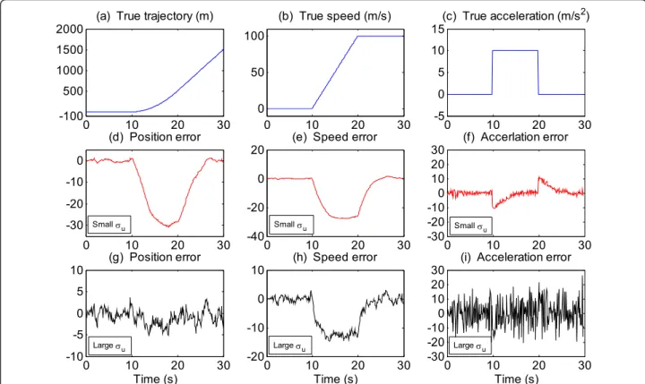
result shows that the sampling time too short will affect the initial convergence rate and diminish the accuracy of the FOSB-based tracking scheme. As compared with the KF algorithm, the location accuracy of the proposed tracking scheme is not always better than the traditional KF-based tracking schemes. That is, for the moving tra-jectory of the second path, the sampling time will influ-ence the covariance scale in (26)-(28), and (34); the shorter sampling time will result in smaller covariance, cause an initial-value problem, and induce larger estima-tion errors. As shown in Figure 8 (Appendix 1), the effect of the standard deviation of the state equation should be considered when the model describing the analytic motion of the MT is based on acceleration noise. Furthermore, the shortage of the speed observa-tion in recursive operaobserva-tions and non-causal nature can lead to a convergence bias if the proposed FOSB-based tracking scheme is used with an improper initial speed value. However, for short sampling time in Figure 6, as the initialization is finished, the results show that the FOSB-based approach is slightly better than the KF-based approach. In terms of Figure 7, as the tracking scheme is based on a fixed-lag smoothing concept with faster sampling frequency, the phenomenon of the

worse initial convergence can be reduced with selecting a more closer initial value or can be overcome with the times of the process cycle based on the inherent mes-sage-passing features to exchange information.

In Figures 5 and 6, as the speed s set to 2 m/s and sampling time set to 1 s, the results demonstrate that more than 90 (60) percent of the non-tracking method had error distances of less than 8.67 (5.40) m for the first and second paths; the estimates of KF-based track-ing scheme had error distances of less than 4.80 (2.98) m for the first path and less than 4.72 (2.94) m for the second path. The estimates of FOSB-based tracking scheme had error distances of less than 4.72 (2.92) m for the first path and less than 4.61 (2.87) m for the sec-ond path. According to the results, the location accuracy of the KF-based and FOSB-based tracking schemes is better than the non-tracking schemes. However, for the linear Gaussian model, the KF-based tracking scheme is an optimal algorithm, and it gives the linear estimator in an MSE sense [27]. Therefore, the location accuracy of the KF tracking results can be considered a reference CDF bound for location accuracy.

For the third path, Figures 9 and 10 present the com-parisons among the non-tracking, the KF-based tracking,

0 200 400 600 800 1000 1200 1400 1600 1800 2000 2200 2400

0 1 2 3 4

S

pee

d (

m

/s)

X-axis

1800 1850 1900 1950 2000 2050 2100 2150 2200

1.5 2 2.5

Number of Samples

S

p

ee

d (

m

/s)

Zoom In

True Speed

FOSB Estimated Speed KF Estimated Speed

True Speed

FOSB Estimated Speed KF Estimated Speed

Figure 6.

0 10 20 30 -100

500 1000 1500

2000 (a) True trajectory (m)

0 10 20 30

-30 -20 -10 0

(d) Position error

0 10 20 30

-10 -5 0 5

10 (g) Position error

Time (s)

0 10 20 30

0 50 100

(b) True speed (m/s)

0 10 20 30

-40 -20 0

20 (e) Speed error

0 10 20 30

-20 -10 0

10 (h) Speed error

Time (s)

0 10 20 30

-5 0 5 10

15(c) True acceleration (m/s

2₎

0 10 20 30

-30 -20 -10 0 10 20

30 (f) Accerlation error

0 10 20 30

-30 -20 -10 0 10 20

30 (i) Acceleration error

Time (s)

Small V_u

Large V_u

Small V_u

Small V_u

Large V_u

Large V_u

Figure 11.

Figure 8Tracking an MT with two different standard deviations.(a-c)true trajectory, speed, and acceleration;(d-f)estimated errors of

trajectory, speed, and acceleration with small standard deviation;(g-i)estimated errors of trajectory, speed, and acceleration with large standard

deviation.

0 1 2 3 4 5 6 7 8 9

0 0.2 0.4 0.6 0.8 1

Location Error (meter)

C

um

u

lat

iv

e P

robabi

lit

y

(a)

0 50 100 150 200 250 300 350 400 450 500

1 2 3 4

Time (second)

A

ver

age Loc

at

ion E

rr

or

(

m

et

er

) _{(b) Average RMSE (1000)}

Observed KF, ST = 1 Sec FOSB, ST = 1 Sec 1 Observed (Without Tracking) 2 KF, ST = 1 Sec 2 FOSB, ST = 1 Sec 3 KF, ST = 2 Sec 3 FOSB, ST = 2 Sec

...

Corner Effect (Peaks) 1

3

2

...

...

...

Figure 7.

Figure 9Comparison of the non-tracking (observed), the KF-based tracking, and the FOSB-based tracking schemes in the third path.

(a)in terms of the CDF of the error distances,(b)in terms of the average location error (RMSE) of 1000 times according to the first 500 samples

and the FOSB-based tracking schemes. The results in terms of the CDF of the error distance of 10,000 sample trials and in terms of the average root-mean-square error (RMSE) of the first 500 sample trials are given in Figure 9a, b, respectively. As the sampling time set to 1 s, the results demonstrate that more than 90 (60) per-cent of the non-tracking, KF-based tracking, and FOSB-based tracking schemes have error distances of less than 4.63 (2.87), 3.04 (1.90), and 3.03 (1.90) m, respectively. In Figure 9a, as the sampling time set to 1 or 2 s, the results show that the location accuracy of the proposed tracking scheme is almost the same as the KF-based tracking scheme. For the proposed FOSB-based tracking scheme, despite the location accuracy, adopting the dis-tributive approach using the prediction-correction recur-sion to implement the location estimator significantly reduces the computational complexity, as shown in Table 4. However, the tracking approach will result in the corner effect generally [8], which is caused by the values of sampling time or the standard deviation para-meter for target acceleration. In Figure 9b, the result shows that the errors of proposed tracking scheme based on one-step fixed lag smoothing are slightly smoother in the moving trajectory of an MT. In addi-tion, the corner effect (the peaks) of the proposed

tracking scheme is slightly larger than the KF-based tracking scheme. That is, the speed of proposed algo-rithm is reformulated by using forward and backward steps, and it further smooth the location state; it results in larger estimation errors around the corners. Further-more, in terms of (35), the MT’s speed and direction of the simulations are based on random acceleration noise and random moving angle. Figure 10a illustrated the simulation result of the samples from 3500 to 4500 within 10,000 trials, the different moving lengths and the random moving angles (or directions) are assumed to simulate the trajectory and direction of an MT mov-ing around hallways in an indoor environment, where the 50 × 50 (m2) square area almost be completely filled with MT’s trajectory after 8,000 simulation trials. Figure 10b is the observation trajectory simulated to be extracted from the measurements of RSSs of WLAN in an indoor environment (cf. [8,14,41]). In addition, in terms of the first 500 samples in 10,000 simulation trials, Figure 11a-l are the original trajectory and speeds, the observed trajectory and speeds, the KF-based track-ing results, and FOSB-based tracktrack-ing results, respec-tively. Figure 11 shows that both the KF-based and the proposed FOSB-based tracking schemes can provide a high degree of accuracy for predicting next-step location

-10 0 10 20 30 40 50 60

-10 0 10 20 30 40 50

60 (a) True trajectory

Length (m)

W

idt

h (

m

)

-10 0 10 20 30 40 50 60

-10 0 10 20 30 40 50

60 (b) Observed trajectory

Length (m)

W

idt

h (

m

)

-10 0 10 20 30 40 50 60

0 10 20 30 40 50

60 (c) Estimated trajectory (KF)

Length (m)

Width (

m

)

-10 0 10 20 30 40 50 60

-10 0 10 20 30 40 50

60 (d) Estimated trajectory (FOSB)

Length (m)

Wi

d

th

(m

)

Figure 8.

Figure 10Simulation results of the location estimation of an MT in terms of the samples from 3500 to 4500 in 10,000 trials.(a)

and speed in tracking paths. In addition, the proposed approach is assumed that the speed observations cannot be obtained, and then the speed is defined and obtained by an MT moving through a displacement during a time interval. According to the simulation results in Fig-ure 11e, f, the observed speeds extracted from location observations cause a large variation and lead to instabil-ity with lower reliabilinstabil-ity. However, for the proposed FOSB-based tracking scheme, the speed estimation is based on weighted reliable information of speed predic-tion and speed observapredic-tion in Step 11. In terms of the correction phase in (10) and oper1 in Table 1, the esti-mation speed will be dominated by the messages with higher reliability. As compared with Figure 11a-i, Figure 11j-l shows that the proposed FOSB-based tracking scheme can achieve an accurate performance very close to the traditional KF tracking scheme, and the tracking results are also very close to non-disturbance data. Con-sequently, when the message-passing rules used for pre-diction and correction phases with improved messages, the oscillation observed in Figure 7 may be caused by the proposed approach, where the performance of the proposed approach is close to an MSE estimator.

In brief, according to the proposed approach and Appendix 1, not only is the FOSB-based tracking scheme derived from Bayesian approach close to MSE estimator, but also the KF-based tracking scheme can be derived from Bayesian point of view based on MSE sense. Namely, the proposed FOSB-based tracking scheme passing the reliable messages between the pre-diction and correction phases can achieve an accurate location very close to the KF-based tracking scheme. Furthermore, the sampling time will influence the state space model and imply the changes of the simulated track. In Figures 5, 6, and 9a, the different values of Δk

are used to generate and analysis in the different curves. These results show that the smallerΔkresults in smaller

location tracking errors. In terms of (15), (16), (34), and (35), the smaller Δkresults in smaller random

compo-nent added to the motion model of state equation. Therefore, for fixed random components σ_kη and σ_kv, the estimation accuracy will be dominated by the mes-sage of the reliable motion model as the state equation is with smaller Δk ; the estimation accuracy will be

dominated by the message of the reliable observation as the state equation is with larger Δk. In other words, -10 0 10 20 30 40 50 60

-100 10 20 30 40 50

60 (a) True trajectory

Width (m)

-10 0 10 20 30 40 50 60 -100

10 20 30 40 50

60 (d) Observed trajectory

Wi

dt

h (

m

)

-10 0 10 20 30 40 50 60

0 20 40

60 (g) Estimated trajectory (KF)

W

idth (m

)

-10 0 10 20 30 40 50 60 0

20 40

60 (j) Estimated trajectory (FOSB)

Length (m)

Wi

dt

h (

m

)

0 100 200 300 400 500

-2 0

2 (b) True X-speed

Spee

d (m/s)

0 100 200 300 400 500

-10 0

10 (e) Observed X-speed

S

peed (m/s)

0 100 200 300 400 500

-2 0

2 (h) Estimated X-speed (KF)

Speed

(m/s)

0 100 200 300 400 500

-2 0

2 (k) Estimated X-speed (FOSB)

Number of Samples

S

peed (m

/s)

0 100 200 300 400 500

-2 0

2 (c) True Y-speed

Spee

d (m/s)

0 100 200 300 400 500

-10 0

10 (f) Observed Y-speed

S

peed (m/s)

0 100 200 300 400 500

-2 0

2 (i) Estimated Y-speed (KF)

Speed

(m/s)

0 100 200 300 400 500

-2 0

2 (l) Estimated Y-speed (FOSB)

Number of Samples

S

peed (m

/s)

Figure 9.

Figure 11Simulation results of the tracking location and speed of an MT in terms of the first 500 samples in 10,000 simulation trials.

when the value of variances or sampling times becomes high, it diminishes the location accuracy of the MT. As compared with the traditional KF-based tracking scheme, the proposed FOSB-based tracking scheme can achieve acceptable location performance and can reduce the computational burden with a slightly large corner effect. Therefore, the approach of the proposed tracking algorithm can work well under the large computational loading conditions.

5. Conclusion

This article presents a forward scheme for location estima-tion and a one-step backward scheme for speed estimaestima-tion with message-passing algorithm to implement the Baye-sian approach. According to the proposed algorithm, not only is a new adaptive weighted scheme used to reduce the computational complexity of traditional tracking schemes, but also the idea of decouplingXandY dimen-sions is used to simplify the implementation for location estimation. In addition, to deal with a shortage of the speed observation in recursive operations, a fixed-lag smoothing concept based on the past and future location information is implemented to avoid the error propagation and then to improve the location accuracy. Namely, the location accuracy of the proposed FOSB-based tracking scheme is weighted and dominated by the incoming mes-sages having higher reliability information of the location and speed between the prediction and correction phases. In comparison, the proposed FOSB-based with the tradi-tional KF-based location tracking schemes, the major dif-ferences between them are the computational load, where the advantage of the former is based on the distributive approach and the decoupling idea for location estimation. For the purpose of increasing the execution speed, the lower computational complexity of the proposed FOSB-based tracking scheme is indeed a valuable improvement for estimating the location of an MT. The simulation results demonstrate that the proposed FOSB-based track-ing scheme, in comparison with the traditional KF-based tracking scheme, achieves close location accuracy. Conse-quently, with the inherent feature of the Bayesian approach, the distributive feature of proposed prediction-correction recursion makes it suitable for practical imple-mentation. To sum up, the proposed FOSB-based tracking scheme, with features of both good location accuracy and low computational complexity, is attractive to use in loca-tion estimaloca-tion for the applicaloca-tion of LBSs in our daily life both indoors and outdoors.

Appendix 1

Kalman filtering

In general, the basic ideas of derivation processes for the KF algorithm are based on three distinctive features of the innovation approach which are linear, unbiased, and

minimum-variance [38,42-44]. However, according to the prediction and correction steps in (4) and (5), if the state space model is linear and Gaussian, a KF algorithm can also be derived and applied to the recursive Baye-sian estimation [31,38]. Let the vector x = [x1, ...,xn]T

consist of independent components i = 1, ..., n. The PDF ofx is the production of the individual PDF’s ofx1, ..., xn; N(x;m,P) is defined as Gaussian density for n

dimensions; then-dimension Gaussian density function is defined by

N(x;m,P) |2πP|−1/2exp{−1 2 (x−m)

T_P−1_{(x−m)},(36)}

wherex,m, and Pare the argument, mean, and cov-ariance, respectively. According to (1), (2), (6), and (7), the KF algorithm can be applied as follows.

f(xk+1|xk) =N(xk+1;kxk,Qk) (37)

h(zk|xk) =N(zk;Hkxk,Rk). (38)

It is assumed that the initial state is Gaussian distribu-tion as p(x0) =N(x0;m0=xˆ0,P0=P0); the distribution

can start from p (x0|z0) = p(z0|x0) p(x0)/p(z0), and then the distribution p(xk|z0:k) is obtained at time k.

Therefore, the cor