ABSTRACT
VANGALA, RAVIKANTH. Design of a Dynamic Quality Control System for Textile Processes. (Under the direction of Dr. Moon W Suh).
An attempt has been made to apply the structural equations published during the last 60 years for designing a dynamic quality control system for dry and wet textile processes that are either continuous or contiguous and are serially connected with time lags.
This new system provides process averages and control limits that are relative to the conditions of the prior processes. According to the new system the changes observed in the prior process will update the process averages and control limits of the current process using the structural relationship between the two stages. By obtaining more accurate control limits, the root causes of the out of control situations will be determined precisely, and unnecessary corrective actions that are detrimental to quality monitoring improvement be minimized. The major research task was to identify all published papers and sort out clearly defined input and output parameters that are essential in determining the structural relationships between the various process stages that are serially connected.
The next challenge was to align and consolidate the multiple equations to a single set at each stage in such a way that a dynamic system can be developed by combining all process steps in sequence, linking all input and outputs parameters. In the jth process, the output Yj is expressed as a function of Yj-1of the previous process and ‘m’ new input factors zj (zj1, zj2, …, zjm);
Design of a Dynamic Quality Control System for Textile Processes
by
Ravikanth N Vangala
A thesis submitted to the Graduate Faculty of North Carolina State University
In partial fulfillment of the Requirements for the degree of
Master of Science
Textiles
Raleigh, North Carolina 08/07/08
APPROVED BY:
__________________________ ____________________________
Dr. Moon W. Suh Dr. Tushar K. Ghosh
Chair of Advisory Committee Member of Advisory Committee
___________________________ ____________________________
Dr. Melih Gunay Dr. Jeffrey R. Thompson
DEDICATION
ACKNOWLEDGMENTS
I would like to express my profound sense of gratitude to my mentor Dr. Moon W Suh for providing me with necessary guidance and support at every step of my Masters study. I am deeply indebted to him for transforming me into a complete engineer and a responsible person.
I am also grateful to Dr. George Hodge and Dr. Abdel-Fattah M Seyam for their constant encouragement and support. I would like to thank Dr. Harold Freeman and the NTC for funding this research. I would also like to thank Dr. Melih Gunay for his ever encouraging words on my performance. I feel greatly privileged to work under the guidance of Dr. Suh and Dr. Gunay.
I wish to thank Dr. Jeffrey Thompson and Dr. Tushar K Ghosh for their valuable feedback and discussions on my thesis.
I am always grateful to my parents and grandparents, with whose constant support, encouragement and blessings I was able to come to the United States to pursue my higher degree. I would also like to thank my brother for his constant belief in me and my capabilities as a performer.
Heartfelt thanks to all my friends at the College of Textiles for their help and support for the past two years and a special thanks to Mr. Rob Cooper and Ms. Tywanna Johnson for their patient support answering all my queries in these two years.
BIOGRAPHY
TABLE OF CONTENTS
LIST OF TABLES ………...…. vii
LIST OF FIGURES ……….. viii
1. INTRODUCTION ………..……… 1
2. REVIEW OF LITERATURE ……….. 3
2.1.Statistical Process Control (SPC) and Statistical Quality Control (SQC) ………..… 5
2.2.Statistical Process Control (SPC) and Statistical Quality Control (SQC) in Textile Manufacturing ……….. 12
2.2.1. SPC in Yarn Manufacturing ………...… 16
2.2.2. SPC in Dyeing and Finishing ………. 18
2.3.Feedback and Feedforward Control Systems in Continuous Manufacturing Industries ………..… 22
2.4.Reasons for Failure of Quality Control Systems in Textile Manufacturing in the Past ……….. 24
3. OBJECTIVES ……….……… 29
4. CONCEPT OF A DYNAMIC CONTROL SYSTEM ……….………...… 30
4.1.Importance of Structural and Functional Relationships for Dynamic Control Systems ………..……..… 36
4.2.Method for the Use of Multiple Structural Equations ………..………….... 38
4.2.1. Fusion Algorithm for Multiple Structural Equations (FAMSE) ….………... 38
4.3.Variance Tolerancing and Variance Channeling ………..… 43
4.3.1. Concept of Variance Tolerancing in Ring Spinning ………..… 43
4.3.2. Methods of Achieving Variance Tolerancing ………..………..… 48
4.4.Advantages obtained using Dynamic Quality Control Systems ………... 50
5. DEVELOPMENT OF DYNAMIC CONTROL CHART &VARIANCE TOLERANCING – APPLICATION IN SPINNING PROCESS ……….
53
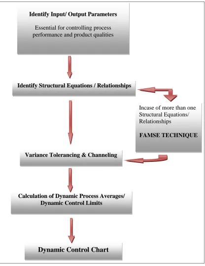
5.1.Approach for the Design of a Dynamic Control Chart …..………...… 58
5.2.Identification of Structural Equations in Spinning on Various Key Factors ………61
5.2.1. Identification of Structural Equations in Spinning for Mass Uniformity..… 61
5.2.2. Identification of Structural Equations in Spinning for Yarn Strength…...… 68
5.3.Development of Structural Equations/Relationships Based on Key Influencing Factors in Spinning ………... 71
5.3.1.Development of Structural Equations considering Mass Uniformity in Spinning as an Influencing Factor ………... 72
5.4.Variance Tolerancing in Ring Spinning - Application Examples …….……..…… 74
5.4.1. Variance Tolerancing for Variation in Mass Uniformity of Spun Yarns …. 74 5.4.2. Variance Tolerancing for Variation in Strength of Spun Yarns ………....… 75
5.5. Design of a Dynamic Control Chart in Spinning ……….……… 76
5.6.Design of Dynamic Control Charts in Other Textile Manufacturing Processes ………...… 76
6. SUMMARY AND CONCLUSIONS ………..………....……..… 78
7. FUTURE WORK ………...… 80
LIST OF TABLES
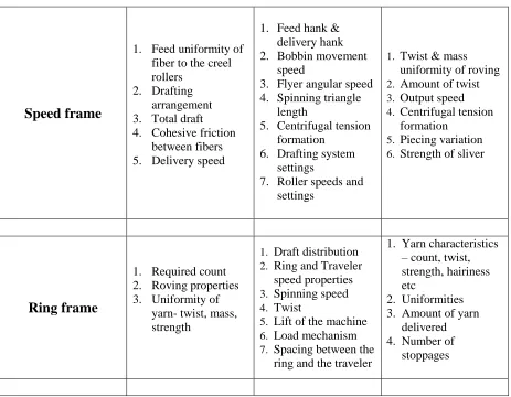
Table 1: Key fiber parameters which influence the processes in Figure 2 ……..…………. 55
LIST OF FIGURES
Figure 1: Schematic Diagram of the concept for Shewhart Control Charts for any
Continuous Manufacturing Process ………...……..….... 8
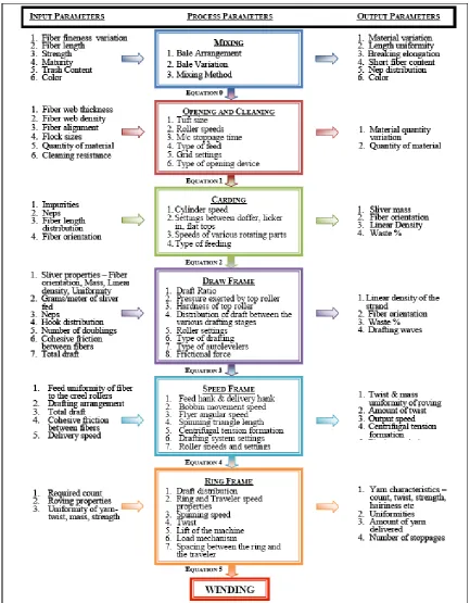
Figure 2:Conceptual Frame for Dynamic Control Limits from Mixing/Blending to
Ring frame via the Structural Relationships Developed …………..………. 32
Figure 3: Schematic Diagram of a Dynamic Control Chart …..………... 35
Figure 4: Schematic Diagram of Inheritance of Variance from Previous Process Stages .... 47
Figure 5: Framework for Structural and Functional Relationships among Key
Spinning Processes ……….……...…… 57
Chapter 1
Introduction
Development of textile science and engineering during the last 100 years has been truly remarkable based on the published research reports and claims. However, as Prof. John W. S. Hearle (UMIST) once said in his farewell seminar at NC State University in 1999, it is quite troublesome to find that only a small fraction of what has been discovered and reported by himself and others is being applied in textile manufacturing operations today [1]. In particular, the structural models and prediction equations published to date are seldom used in quality and process control practices in the US or elsewhere. A large number of scientific and engineering equations remain unused in practice, whether understood or not. Also, it is often startling to discover that textile-manufacturing operations throughout the world seldom make use of the vast amount of advanced technical information accumulated during the last 50 years for their quality-control and improvement efforts.
statistical approaches using regression and correlation analyses in place of finding the true underlying structural relationships. The estimated coefficients thus found from specific populations and operating conditions are often highly volatile and unstable. Furthermore, proving a statistically significant relationship does not necessarily guarantee the existence of a true cause-effect relationship.
Over the years, textile producers and manufacturers have made huge investments in the quality control department but are unfortunately it neither reduced costs nor increased benefits to its maximum potential. This is mainly due to the use of control systems that are static and inflexible for accommodating the complex, dynamic and interactive nature of textile production environment. Frequent false alarms and unwarranted process calibrations based on the “single stage control algorithms”, often built in the manufacturing equipment, have resulted in loss of production time, materials and consequently profit [3].
Chapter 2
Review of Literature
One of the oldest industries, which fulfill the basic needs of mankind, is the „Textile Industry‟. It is believed that the first traces of textiles (scraps of linen cloth) were found in the
Egyptian caves around 500 BC [6].
In the textile industry, the concept of quality control always has its own importance, centralizing and standardizing textile production occurred as early as the Zhou Dynasty (11th to 8th Centuries BC, China). This dynasty had very explicit stipulations and standards for silk and cotton fabrics and textile producers who didn‟t meet these exacting standards were penalized and punished. The quality standards were so highly observed that even a decree was passed which stated: “Cottons and silks of which the quality and size are not up to the standards are not allowed to be sold on the market.” They even incorporated separate
warp and weft standards for silk in the north and south because of differing weather and humidity [8]. In the West, an early regulation for quality assurance in the textile trade dates back to the 14th century. In Germany a special practice called „Tuchshau‟ (Showing of Cloth) was followed, where a panel of expert inspectors along with an equal number of city council members supervised the entire manufacturing process starting at the loom. No piece of cloth could be sold unless it was produced under this supervision [9].
The concept of „Quality‟ has been a topic of intense interest today. „Quality‟ has been the buzz word among managers and executives in contemporary organizations and Feigenbaum [10] once said: “Quality is the single most important force leading to the economic growth of companies in international markets.” In a survey conducted in the year 1990 [11], executives ranked the improvements of service and product as the most critical challenge facing U.S. business.
and/or Exceeding Customers Expectations (Gronroos, 1983; Parasuraman, Zeithaml & Berry, 1985) and Loss Avoidance (Taguchi, cited in Ross, 1989).”
According to Kadolph [12], some view quality as a factor or a group of factors that can be controlled by inspecting finished products. In these inspections the satisfactory or acceptable products which pass are sold at normal prices while unacceptable products are sold as seconds at a lower price. But to guarantee 100% quality through examination is quite impossible for any manufacturing industry and especially in textile industry, the inherent variations coming from various stages during processing make it further difficult to guarantee quality at all levels and stages. Hence, manufacturers prefer controlling the system that produces the product to control of products.
Whether the companies are involved in producing materials or finished products, they are involved directly with the customer. According to Atilgan [13], the production of quality goods consistent with standards with the aid of standardized quality control systems has not only increased the revenue of the manufacturers but also the world trade. Hence, there is a need for better quality and higher productivity.
2.1
Statistical Process Control (SPC) and Statistical Quality
Control (SQC)
time production and some of these statistical quality control methods were even classified as military secrets. Later, Kaoru Ishikawa [14], a well-known Japanese quality philosopher speculated that the Second World War was won by quality control and by utilization of statistical methods.
Shewhart [14], considered as the father of Statistical Process Control (SPC) and inventor of control chart technique, believed that any industrial process could be brought into statistical control by defining the limits of random variation for any aspect of a worker‟s task. The modern quality movement is said to have started on May 16, 1924, when he sent a one page memo to his higher authorities describing a method for improving the quality of telephone manufacturing using statistics which also included the drawing of probably the first control chart wherein he defined the control chart as: “A decision-making device that gives the user information about the quality of product resulting from a manufacturing process.”
which is designed to be implemented in real time after the baseline and control limits have been established.
In the case of Shewhart Control Chart procedure [15], the parameters of interest are the average and standard deviation and the upper and lower control limits are symmetrical about the average. If M is a control statistic (say), its mean will be μM and standard deviation
σM. Then the Central Line (CL), the Upper Control Limit (UCL) and the Lower Control
Limit (LCL) are calculated as follows: UCL = μM + kσM
CL = μM
LCL = μM − kσM
where k is the distance of the control limits from the central line, expressed in standard deviation units.
Of late, there have been many articles written on the subject of SPC/SQC as a new technique for transforming management. Although these researchers claim novelty in their concepts and techniques, these are not new. Deming [16] advocated fourteen key principles of management for transforming business effectiveness over forty years ago and encouraged the use of basic statistical formulas to identify, control and ultimately eliminate special causes of variation in the process, referring to these methods as Statistical Quality Control (SQC). According to him, „statistical thinking is critical to improvement of a system‟. His so-called 14 principles have been the impetus for the widespread use of data and statistical methods in process industry today.
Deming [14] identified several different charts for use in achieving statistical control of a process and most manufacturing companies implement Deming‟s SPC/SQC via use of the control chart. The most frequently used charts are:
Cause and Effect – A chart used to examine factors that influence a given condition
Flow Chart – A chart used to delineate the steps in a process
Pareto Chart – A chart used to determine priorities indicating the most significant factors
Trend or Run Chart – A plot of the data used to determine patterns of behavior
Histogram – A chart used to measure the frequency of occurrence
Scatter Diagram – A chart which demonstrates the relationship between two variables
SPC/SQC assumes that every process has variation and control charts help us to identify, analyze and control those variations in each process. As mentioned earlier, a process is said to be in control when no points fall outside the upper and lower control limits and there are no special patterns observed in the points. SPC/SQC seeks to minimize that variation via these charts by assisting us in identifying and ultimately deciding which control actions should be taken to eliminate the source of that variation. The successful SPC/SQC program utilizes statistics to identify and eliminate special causes of variation, thereby driving the process into a steady state of control. Once control has been achieved, the control charts should continue to be used to monitor the process so that aberrations can be quickly identified and resolved maintaining a steady state or controlled process.
In any production process, there exists certain amount of inherent or natural variability depending upon the number of process and input variables. The variability in quality that occurs in an actual production process should be either „error‟ or „natural/inherent variability‟. Sources of variability which are identifiable and preventable are called as „assignable causes‟ or „special causes‟ of variation. Common examples of such causes are improper functioning of machines, employing wrong methods, faulty raw material etc. Generally, these „assignable causes‟ are considered to lie outside the process and contribute significantly to the total variation of the process performance. Although, the variation in such cases is usually unpredictable, it can be very much explainable after the causes have been observed.
each interval of time. These variations are thus very much predictable and are labeled as „noise‟ because there is no real change in process performance. Sometimes, „noise‟ cannot be traced to a specific factor/cause, and it is therefore, either uncontrollable or unexplainable although very much predictable. The amount of variation from the target in the process thus depends on the strength of the noise and has a huge impact on the controllable process factors/ parameters. Variation is created by both common causes (which contribute to controlled variation) and assignable causes (which contribute to uncontrolled variation). The term controlled variation as explained by Shewhart [17] as follows: “A phenomenon will be said to be controlled when, through the use of past experience, we can predict, at least within limits, how the phenomenon may be expected to vary in the future, where prediction within limits means that we can state, at least approximately, the probability that the observed phenomenon will fall within given limits.”
the process variability engineering functions have to be used. If the only variability present is due to common causes and all special causes are absent, the production process is said to be in a state of statistical control. Using the probability laws which govern the stable state of control, special cases can be detected such as the special or assignable causes increasing the variability beyond the level permitted by the common or chance causes.
Over a period of time variations owing to special causes are bound to occur due to changes in raw material or operatives or sudden machine failures etc. Therefore the process is usually sampled over time, either in fixed or variable intervals. The presence of special causes can be monitored by considering a control statistic such as the mean ( ) of a sample of units taken at any given time. The approximate probability distribution of the control statistic can then be used to define a range for the inevitable common cause variation, known as control limits. This allowable variation can also result in false alarms. That is, even when no special causes are present, we may be forced to look for the presence of special causes.
Hence, it is necessary for the technical person to be familiar with the statistical techniques and also for the statistician to have some knowledge of the production processes.
2.2
Statistical Process Control (SPC)/ Statistical Quality Control
(SQC) in Textile Manufacturing Industry
Shewhart Control Charts, Deming practices for Continuous Improvement and the Juran Team Approach to Quality Improvement.
According to Bona, textile quality control often involves keeping output of individual processes in control though the use of Shewhart Control Charts [19] and in a world of global marketing, compliance with international standards for quality in conjunction with various international certification standards has become of paramount importance to manufacturing companies in America. American textile companies are more than ever faced with the challenge to produce better quality products, faster and at reduced costs. These companies are making every effort to achieve control of their manufacturing processes from dyes and chemicals usage to machine efficiency to operator performance; from inventories to on-time deliveries. Every aspect of the process is being analyzed in an effort to improve quality and to optimize productivity.
In textile manufacturing industry, loss resulting from high variability can be defined as a loss to society which can be associated with every product that is shipped or transferred to a consumer. The user of the fiber is the spinner, the user of yarn is the weaver, and the chain continues down to the consumer of the apparel or any textile product. Thus, each intermediate operation in a textile manufacturing line should be considered as an independent society even though they are contiguous in nature.
rules are referred to as acceptance sampling. In simple terms, they represent a set of communication tools between the user and the producer.
The second generation of quality assurance development in textile manufacturing started with the advent of Statistical Process Control (SPC) Techniques. Online quality control systems have been traditionally used to describe the statistical process control concepts such as control charts, cause and effect diagrams, process capability studies etc., and this development led to the successful minimization in rejections. The main objective of the SPC programs was to keep the variability of a process or product within the customer specification limits.
In recent years, different sectors in textile industry started implementing SPC as the technology in textile machinery and product specifications have been changing rapidly imposing new quality demands. Also, increasing computing power, availability of numerous SPC software programs and the increasing competition at both local and international levels permit real-time control charts. The first step in the setting up of a quality control system in textile manufacturing is the determination of where the major variations are occurring and of what characteristics should be controlled.
Region” and “Out of Control” points so that the over-all quality records of a department can be compared from week to week [21].
The knowledge of quality control chart methods facilitates the planning of the comparison. The control chart techniques emphasize about the principles to follow in sampling i.e., the use of frequent small samples instead of infrequent large ones, rational subgroups and grouping of data on the basis of production. As mentioned earlier, the variations are labeled as „noise‟ and the noise factors in textile manufacturing can be broadly divided into two categories: External and Internal. External noise includes the factors which are not a part of processing but still affect the process such as temperature, humidity, dust etc. Internal noise includes mainly product and manufacturing factors such as draft variations, twist variations, short fiber content etc.
In the recent past, revolutionary developments have been made in textile technology which led to wide scale industrial applications of textile products. These applications call for a new approach to quality based on design aspects but it is believed that implementing the design aspects in quality programs is more expensive than monitoring and re-adjusting the process as variation of assignable causes occurs [23].
2.2.1 SPC in Yarn Manufacturing
The yarn manufacturing area of the textile industry offers a wealth of data for statistical analysis. Articles on the statistical quality control of textile yarn manufacturing products such as sliver, roving, and yarn date back to the late 1940s and 1950s. In these articles, the emphasis is on product quality and defect detection rather than on defect prevention through process control and quality improvement. Unfortunately, even in those articles which focused on quality control, there has been hardly any usage of the structural equations or relationships between the input and output factors.
For faster feedback, some yarn manufacturers are beginning to move some test equipment (e.g., yarn boards, reels, skein winders, and balances) to the production floor. This is a process-oriented quality feedback and allows the operator to better yet would be a move toward determining key processing factors that affect the key internal and external customer requirements of the outgoing product and then controlling and optimizing these factors.
Inspection for spun yarn manufacturing is directed toward finding defects such as thin places, thick places, or slubs that can cause further problems in yarn preparation or fabric forming. In addition, it is done to reduce the chance for off-quality fabric resulting from irregular yarns. Warp yarns for weaving are typically graded more critically than filling yarns or knitting yarns. Package build, knot quality, and package density are other factors graded during inspection to ensure good running performance in later processing.
Given the quality levels of the past, the need for yarn inspection is warranted. It is however, very costly, and when unacceptable levels are found and lots rejected, losses are great in terms of raw materials, wasted manpower, and improper utilization of processing equipment. Furthermore, the cost of unproductive inspection is far too high. As the focus moves toward process control, defect prevention, and quality improvement, the need of inspection markedly reduces.
through over-control than would occur were the process controlled manually through the use of control charts.
2.2.2 SPC in Dyeing and Finishing
The process of dyeing a textile fabric has historically been one of the most monitored and controlled processes in the manufacturing chain. The finishing processes, however, are at the other end of the spectrum with fewer controls and heavy reliance upon inspection and testing. In fact, most mechanical finishing processes are considered to be much more art than science. This leads to a great deal of subjectivity whenever evaluating finishing processes.
Dyeing Processes
Process parameters such as temperature, pH, rate of temperature rise and cooling, etc. for the dyeing process have been widely known, documented and monitored for many years.
Different levels of control equipment for dyeing have been readily available for the past 25-30 years. However, as is in the case in spun yarn manufacturing, controllers for dyeing
have historically used predetermined set points and not statistically calculated control limits to make adjustments, signal alarms and /or stop the operation. This leads to an over-control situation and increased variation for the process.
In order for dye-houses to effectively use the monitoring and controlling equipment available today, the following items must be addressed:
Statistical control of raw materials (including dyes, chemicals, water, fabric, etc.)
Use spectrophotometers to establish dye formulas, determines color additions, and evaluate the final shade, or color of the fabric.
The processing technique whether employed in the laboratory or in the plant are subjected to a greater extent to variation when the same operating sequences are repeated. Also, the resultant degree of variation in the quality of a manufactured product, and the tolerances resulting therefore, are determined largely by experience and are only rarely defined on a statistical basis. However, this is a necessary requirement for optimization of the production sequences and therefore it is very essential to improve the accuracy by means of statistics.
Dyeing is considered as one of the most critical, complex and costly operations. In dyeing there are many sources of product variation which can be attributed to many factors including:
Material Variations Variations in Chemicals
Variations in preparation of the substrate for dyeing Procedural Variations
The above factors leading to variation in dyeing can generally be classified into two classes: 1) Process Variations and 2) Raw Material Variations. Raw material monitoring is very essential to accomplish process optimization. If raw materials vary, then process optimizations are nothing more than adjustments to a fluctuating input, and the result is continual change with little improvement.
production, are the direct result of the inherent limitations of open loop control systems when applied to the dynamic process of dyeing.
Gilchrist et al. [24] developed a mathematical model to predict the uneven levelness in a dyed yarn package and used the model and in-line measurements of the dye liquor concentration and liquor temperature feedback control to achieve and maintain a set rate of dye exhaustion in a pilot scale dyeing machine. The mathematical model uses a mass-balance approach to calculate the dye present in the yarn package and in the liquor and differential equations to describe the rate of dye adsorption. They defined the quality of the final dyeing in terms of uneven levelness in color are measured by the dye deposition error across the package. This simply the difference in the amount of dye deposited on the inside and outside of the package and is related to the visual color difference. This simplified structural model of the dyeing process is used to predict the uneven levelness at any time during dyeing cycle based on the measured rate of exhaustion, liquor flow rate, total liquor volume, etc.
--- (1) where A = internal radius of package, B = external radius of package, r = radius of interest, V = total dye bath volume, Vs = dye liquor entrained in package, t = time, M (r,t) = amount
of dye on fiber at radius r, time t, K (t) = rate constant of dyeing, F = flow rate, C (t) = dye bath concentration at time t, K‟ (t) = overall rate constant of dyebath, ω (t) = ratio of rate constants = , and Є = porosity of yarn = 1 –
where Dt – Total amount of dye to be adsorbed by the fiber, Z(t) – Incremental deposition
error
A significant application of the prediction method [25] was made in the determination of limits of accuracy in the control of the dyeing process. To produce a right-first-time product, process control is essential for dyeing. Any failure to control the dyeing operation may be disastrous for the resulting dyeing quality. In a dyeing process, the limit of each step in the process is reflected in the results of final dyeing. The limit of accuracy is the definition of a process limit such that the accumulative effect of each variable gives an end product within the tolerance level. Hence, the dyer has to know the tolerance levels for specific variables of specific recipes.
To determine the total color sensitivity ( of a dye recipe, based on the recipe color sensitivity (S) and the changes in lightness, chroma and hue (
--- (3)
where, ; ; ; Li, Ci, and Hi indicate respectively, the change
caused by a unit percentage change of a parameter for lightness, chroma and hue and is the change of a parameter i (i.e., concentration c, temperature T, time t, and liquor ratio r respectively);
Finishing Processes
finishing is often defined as any operation that physically manipulates the fabric with mechanical devices to improve the fabric appearance or performance. Process control parameters for both chemical and mechanical finishing are known, but the evaluation methods used for both areas tend to be very subjective. For most finishing processes, a key measurement is the way the fabric feels. This is called the hand of the fabric and is measured by having people touch the fabric and giving it some type of subjective description. This is why the finishing processes are often described as “an art rather than a science.”
In the Textile Finishing Industry, not only are efficient technical plants required but also an extensive flow of information between suppliers and customers is required to achieve better reproducibility of manufacturing processes and thus a better uniform product quality. Accuracy in this case means that the production process takes place within narrower limits and that it is capable of adhering to these limits with a high degree of probability.
2.3
Feedback and Feedforward Control Systems in Continuous
Manufacturing Industries
As mentioned earlier, the consistency of the product quality has become a major deciding factor in the highly competitive industrial markets. Regardless of the changes of the environment, the duty of engineers is to ensure that the controlled product quality lies within the specification limits. This has led to an intensive research in the field of monitoring and assessment of the control-loop performance in continuous manufacturing industries including the textile manufacturing industry during the last decade.
continuous manufacturing industries such as the textile industry. Desborough and Harris in 1993 [26], used analysis of variance table to investigate the variance contributions due to
disturbances and controllers for a feedback/feedforward system. In the year 2000, Huang et al. [27] extended the Minimum Variance Control (MVC) methods to feedback/
feedforward systems and based on linear time invariant assessment techniques, the time varying minimum variance benchmark in feedback and feedforward control systems was developed by Olaleye et al. [28] in 2004. Several other researchers like Petersson et al. [29], Stanfelj et al. [30], Sternad and Soderstrom [31] also tried to extend the MVC theory to define feedforward/ feedback performance. However, feedback control is not a new concept. Its first use was documented when James Watt used a fly-ball governor to control the speed of his steam engine [32]. The technique developed slowly at first and has evolved from the use of pneumatic and electrical devices to a wide range of intelligent digital devices from various vendors which are all integrated to provide real-time control actions in response to variations in the process.
desired specification levels, the control system makes every effort to automatically compensate via feedforward, feedback or a mixture of feedback and feedforward control.
A feedforward system measures the input disturbance directly and with that knowledge takes measures so as to eliminate the impact of the disturbance on the process output. This system is often used in a combined feedforward/ feedback control system. Depending on the controlled output, the feedback-only effect or the feedforward-only effect contribute to the output variance of the feedback/ feedforward system. The feedback loop variance can be expressed as the sum of the feedback invariant term and the feedback-dependent term. Generally, it is difficult for operators who supervise the process to determine which parts of the system are defective. Hence, a diagnostic tool is required to assist the operators in keeping the system at the normal operation and in finding out the possible faults. The measured output consists of the disturbance effect from unmeasured disturbance in the feedback loop and from measured disturbance in the feedforward loop. Any fault in the control elements will violate the output response. The diagnosis is to analyze the measured output data and to find out the fault causes when the process faults come from the control elements.
2.4
Reasons for failure of quality control systems in textile
manufacturing in the past
is mainly due to the use of control systems that are static and inflexible for accommodating the complex, dynamic and interactive nature of textile production environment. Frequent false alarms and unwarranted process calibrations based on the “single stage control algorithms”, often built in the manufacturing equipment, have resulted in loss of production time, materials and consequently profit. In case of an out-of-control situation, the backtracking of the problem source naturally begins with the last machine where the problem is caught [2, 19]. This is known as feedback control, which often accompanies instability with a tendency for over-control or unwarranted calibration.
In addition, a feedback control in textiles often leads to disappointing guesswork rather than an effective corrective action due to 1-to-N nature of manufacturing processes [34]. Thus, use of a static target reference in a continuous, dynamic textile process causes frequent false alarms when the changes in process averages originate from the prior process stages. To remedy this difficulty, a dynamic EWMA control chart procedure [35, 36] can be employed. However, this procedure was somewhat effective only for short-run process control situations as it forces us to examine only the current process average against the target with no reference to the biases generated by the prior processes [37] indefinitely. This undoubtedly is a terribly inefficient control process completely void of structural relationships already known for the causes and effects.
systems while describing the main reasons for failure of the past textile research in quality control and improvement as follows:
Forward Prediction Equations: Predicting yarn and fabric properties based on fiber and processing characteristics is a typical example of forward prediction equations. This knowledge base, while critical for general optimization, has not been utilized primarily for three reasons:
the prediction equations are not applicable for specific choices of raw materials, machinery, and processing conditions, thus accompanying large amounts of bias and errors
the forward-prediction equations are useless in tracing back the responsible factors and processing conditions that produced the specific „out-of-control‟ situations on a daily basis
the predictions usually link no more than two stages, with no capability to go back beyond the immediate past step
The fact that forward-prediction equations are inadequate for a backward projection leads textile quality control to disappointing guess work rather than effective corrective action. In summary, forward prediction equations are both incomplete and disjoint for making a truly satisfactory forward prediction, while the ultimate equation, even if it is found, cannot move backward to a set of unique prior-process conditions which produced the specific outcome.
the input or predictor variables. Depending on the functional forms, the variances and/or coefficients of variation (CV) of the output factors are often found to be much greater than those of individual factors. As the complexity of the functional form and the number of predictor variables increase, the precision of the factor to be predicted becomes extremely low. When this reality is added to the introduction of the „process variance‟, it is not surprising at all that the multitudes of forward-prediction equations are seldom used in quality-control and quality-improvement practice in textile manufacturing.
Sample Sizes and Sampling Practices: In manufacturing quality control, the purpose of the sampling is often to detect the out-of-control situations in the process averages that change with time. Sampling intervals and sampling frequencies are as important as the sample sizes and the sampling fraction. Based on these, the random-sampling and testing practice which prevails now is grossly inadequate and superfluous. None of the sampling/ testing methods for raw materials, intermediate fiber assemblies, yarns and fabrics have been time-aligned or location-specific to provide a meaningful analysis. When random samples are taken at infinitely small fractions and analyzed for statistical correlations only, the likelihood of either confirming an existing correlation or pinning down the root causes of the observed deviations becomes extremely low.
An example may be drawn from the testing of cotton bales by using an HVI (High Volume Instrument). Although each and every bale is tested for uniform laydown and blending purposes in the USA today, 2000 cotton fibers may not adequately represent the entire bale of a single test beard consisting of roughly 500 lb or 272,000 g. If every fiber is assumed to be 1 in. (2.54cm) long and to have a fineness of 4 micronaire units (i.e. a linear density of 0.157 tex), a bale of cotton contains 56.7 billion of fibers, or enough to go around the earth 36 times when the circumference of the equator is estimated at 40000 km. In terms of the sampling fraction, the HVI testing is equivalent to testing one out of every 28.35 million fibers. Whereas the testing of yarn and fabric properties is somewhat better than this, there exists little chance of isolating an out-of-control situation based on this type of current sampling and testing practice.
Chapter 3
Objectives
1. To develop general theories and design an effective dynamic process and quality control system which would be applicable to textile manufacturing processes, especially for staple spinning processes as a model case.
2. Survey and analyze the structural/functional relationships in the production and control of ring-spun yarns and consolidate them to form a final set of equations for the design of a Dynamic Quality Control System for a few control factors.
3. Develop a concept for an algorithm (FAMSE) aimed at streamlining a set of multiple structural/functional equations that may be similar to each other, redundant, incompatible or contradictory to each other.
4. Apply the variance tolerancing method developed by Suh et al. [4, 5] to the variance of an output function based on the variances of the input and output parameters selected for the spinning processes in order to establish the dynamic control limits in continuous time domain.
5. And finally, to establish the “dynamic process average” and the “dynamic control
Chapter 4
Concept of a Dynamic Process Control
System
remedy to such a situation is to widen the control limits for all of the subsequent stages. By continuing the practice, however, all control limits become so wide to make the so-called statistical limits useless.
As mentioned earlier, a new dynamic quality control system is one of the most attractive alternatives to the current practices in dry and wet textile processes. A Dynamic Control System can be defined [39] as a continuously-acting control system which responds to normal and abnormal system conditions or events so as to enhance the system stability by acting upon one or more system quantities as determined by measurement of one or more system parameters.
It is accomplished by combining the known structural models linking the process input to the output variables through time-dependent statistical models similar to EWMA and on-line computer simulations [35]. The discrete textile processes are linked through the structural equations via variance channeling as already demonstrated by Suh and Koo [4, 5].
The concept of a “dynamic control chart” procedure incorporates the following: Additive effects of the system biases
Magnification of biases on subsequent process stages through “structural or functional relationships”
Additive random errors
Feedback control mechanisms for excessive biases and errors
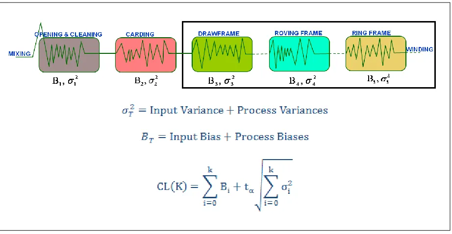
In the continuous process type of manufacturing, such as ring spinning, each process stage is tied to the next as the output material from the previous processing stage is the input feed for the subsequent processing stage, as shown in Figure 5. Generally the input error σ02
speeds, humidity, actual drafts, and mechanical imperfections of equipment add variation. In the case of ring spinning, variation is usually composed of several distinct sources such as the variation inherited from the previous process, within-spindle and between spindle variations, within frame and between frame variations etc.
Each (i) of the k stages is assumed to generate certain amount of bias (Bi) and random error (σi2) inherently. The input bias B0 may or may not be zero as the raw material that
enters into processing is not perfectly uniform. At kth stage, the total bias (BT) must be
separated from the random component σT2, the total error variance. This is the only way the
kth stage control limits can be examined independently of the expected total bias.
Figure 2:Conceptual Frame for Dynamic Control Limits from Mixing/Blending to
The two key points to be considered for the construction of a dynamic control chart are: Estimation of the biases based on the “structural relationships”
Estimation of the process variance at each stage and the total upto a given stage to provide “dynamic control limits.”
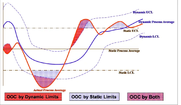
The traditional static process average and the corresponding control limits are now coupled with the dynamic process average and its control limits which reflect the biases of the previous stages. The decision scheme is as shown in the Figure 3. One important point is that the out-of-control situation based on the static limits has to be “swallowed” even if it is neither desirable nor acceptable. The only remedy would be to correct the previous stage processes through the known structural relationships via feedback algorithms.
The graphics can be modified in various ways in order to make the dynamic control most practical and easy to understand. The importance is to understand and quantify the inter-dependence of all the processes in advance in order to make the process control system more responsive to the ever-changing conditions of the process.
Case A: The actual process average is found to be out of control with respect to the static control limits. This case is where no corrective actions may be justified even when the process average exceeds the static control limits.
Case B: The actual process average is found to be out of control with respect to the dynamic control limits. This case is considered to be the case where a corrective action in the particular stage can be justified independently of the biases generated prior to that stage.
4.1 Importance of
Structural and Functional Relationships for
Dynamic Process Control Systems
on-line or off-line depending on the processes involved and the need. The Out-of–Control decisions can be made using both the static limits and the dynamic limits.
4.2
Method for the Use of Multiple Structural Equations
Almost in each and every continuous manufacturing process, we find many structural equations for various intermittent stages in processing in the literature which exist in different forms with varied number of input and output parameters. As each research finding from each researcher around the globe yields new and mostly a different structural equation sometimes we may even find hundreds of equations on the same processing stage or sometimes we may find hardly any structural equation on a particular processing stage. Also, sometimes we may face a situation wherein we come across the same equation written in different forms by various researchers. Sometimes, it even depends on the environment and the place the research is being carried. From a researcher with high mathematical skills it is obvious to expect a complex mathematical structural equation involving many processing parameters that affect the process at that stage. Hence, it becomes a very tough task to pick the right and the best fit equation among those as each one has its own merits and de-merits.
In order to find the right structural equations and to consolidate equations into one final equation when there is more than one structural equation at each stage of spinning, we have developed a novel concept called the Fusion Algorithm for Multiple Structural Equations (FAMSE) Technique which is used to consolidate the multiple structural equations of any form.
4.2.1 Fusion Algorithm for Multiple Structural Equations (FAMSE)
for every processing stage for most of the manufacturing process. Especially in the case of ring spinning process at every stage of processing we find many structural equations in the literature which can be used to determine the variation in mass, irregularity, strength, uniformity etc. It is a tough task to pick the right and the best fitting equation among those as each one has its own merits and de-merits. Sometimes the same equations are written in different forms by different researchers or they have to be slightly modified so as to make it into a feasible one. As mentioned above, we even find contradictory statements or equations by researchers and when we have to pick the one that fits the best, we cannot decide or choose one among those depending on their proofs or explanations. Also the number the input factors vary for almost each and every structural equation.
In order to consolidate N multiple structural equations, that may exist between the input and output variables, where the output Yj at jth process stage is expressed as a function of Yj-1 of the previous process and „m‟ new input factors zj (zj1, zj2, …, zjm), the new algorithm (FAMSE) being developed obtains one structural equation from the „N‟ original sets. Thus, when we find „N‟ structural equations with certain number of factors, each structural equation is re-written in Polynomial form. These polynomial functions with same input terms are consolidated into one equation which is of the form
,
where
11 12 21 22 23
31 32 33 34
1 2 3 4 5
0 0 0 .... 0 0 0 .... 0 0 .... 0 . . . .... . . . . .... .
....
N N N N N Nk
N k
a a a a a
a a a a
a a a a a a
Hence in order to consolidate multiple structural equations and to determine the best fit equation a new algorithm is developed called the „FAMSE Technique‟. After the „N‟ structural equations are re-written in suitable polynomial form they are consolidated in various ways/methods such as by equating, by mere sub-merging, by simplifying them into congruent forms and solving them using various simultaneous equations solving techniques
and using mathematical computational tools/software such as MAPLE, MATLAB, TK SOLVER!, etc.
4.2.2 Components of FAMSE
There are two significant components in designing the fusion algorithm.
1. Factor Decision: Number of factors to be considered is an important aspect in the
2.
Consolidation: As mentioned earlier there would be a situation wherein many polynomial functions with same/similar number of input terms would be identified and they have to be consolidated into one equation. This can be achieved in various ways. For example: By equating/ By mere submerging/ By simplifying into congruentforms/solving using mathematical computational tools such as Maple, Matlab, TK Solver!
4.2.3 Various Stages in FAMSE
1. Redundancy Check
The first step in FAMSE is to check if more than one equation with identical X-variables are redundant even with different coefficients for X‟s when there exist internal functional relationship(s) among X‟s.
As a simple example:
Y = 2X1 + 3X2 + 3X3 --- (4)
Y = 2X1 + X2 + 9X3 --- (5)
with X2 = 3X3
Now, when 3X3 is substituted in the place of X2 equations (4) and (5) turn out to be
the same. Hence, they can be considered as redundant equations and one of them can be eliminated.
2. Congruency Check
substitutions, etc. As an example for congruency check, a couple of equations which were surveyed from the literature for the mass variance at mixing stage in spinning process are considered. (A detailed explanation has been given in the next chapter (section 5.3) about the identification of these equations.)
--- (6)
--- (7)
--- (8)
The equations (6) and (7) above are congruent and when a term in Equation (7) is substituted with Equation (6), we get Equation (8). Thus, two equations are consolidated into a single equation
3. Fusion Modeling
When the “cleaned up” equations are in various functional forms, they have to be “fused” into similar type of structural equations using known algorithms such as Taylor‟s series expansion and Maclaurin‟s series expansion.
Consider the following case where the function with the term ( ) has to be computed.
where K1, K2, K3 are arbitrary constants.
Expansion of ( ) using Taylors Series around “a”,
+ + …
--- (9)
4. Simulation
In order to solve simultaneous equations, various mathematical computational tools such as Matlab or Maple or TK Solver! etc can be used. These computational tools use simulation techniques to solve the simultaneous equations.
For Example: Consider
--- (10)
--- (11)
--- (12)
4.3
Variance Tolerancing and Variance Channeling
4.3.1 Concept of Variance Tolerancing in Ring Spinning
Suh [2] pointed out in his paper that in textile manufacturing, large variations in
materials and processes in addition to the complex structural relationships that are largely unknown or difficult to verify in the presence of huge process variations. In this situation, an improvement in signals cannot be easily verified without reducing and estimating the random noise.
Suh and Koo [4, 5] pointed out that much textile research in the past has been devoted to „forward prediction and characterization‟ of physical properties such as strength, evenness, uniformity etc through various modeling approaches. These models have long been using forward prediction equations to estimate the average pattern of output characteristics from available averages of input characteristics. However, the prediction as well as the accuracy of characteristics to be predicted becomes extremely low as the complexity of the
functional form and the number of predictor variables increases. This is due to the non-uniform and confounding response pattern of the output variable over the entire ranges
of the predictor variables that are often highly correlated among them. When this reality is added to the large variance introduced at each process stage (process-induced variance), it is not surprising at all that the forward prediction equations are neither precise nor accurate enough to control or improve the qualities in textile manufacturing.
In developing a forward prediction equation, difficulties are often due to the „trivial many‟ components that inhibit formulation of an exact functional relationship. In estimating the variance of a response variable with high precision, therefore, only the „vital few‟ must be chosen for variance tolerancing. This may be accomplished in two steps:
finding a geometric, probabilistic, or structural model that is capable of estimating the variance of a product characteristic defined by its intrinsic components.
The definition of an intrinsic component is the component which is measurable or countable and is measurable or countable and is structurally imbedded for explaining the variance of Y. The intrinsic component can be an input material characteristic, a geometric or structural factor. They can be filtered by using such as Pareto analysis of variance components. For tensile strength of a yarn, fiber length, strength, fineness and yarn twist can be the intrinsic components and in the case of tensile strength of a fabric, yarn tensile properties and the density of weave can be the intrinsic components.
Conventional statistical tolerancing methods while effective in many well-defined processes are inadequate in many ways for textile products and processes. The control and improvement strategies for textile process qualities will have to come from better analyses of variance on the input and output variables imbedded in simplified and verifiable structural relationships.
Statistical Tolerancing techniques can be used to determine the probability distributions of output characteristics from a set of input component variances when the structural cause and effect relationship is known functionally. This technique, however, is not easily applicable to textile products and processes, where reliable functional forms of the structural relationships are either not known at all or only partially understood.
characteristic into relevant sub-components. Then a set of variance ranges are set up for the sub-components. Applying these, out-of-control situation in the output characteristic signifies that there exists a set of input variances which were significantly deviating from the norms established. By examining the ranges for the input sub-components one at a time, it is possible to comb out the responsible factors and/or processing conditions that produced the specific out-of-control situation. Securing statistical distributions for suitable input quality components with the objective of quantifying a desirable output quality characteristic statistically is practically more meaningful as well as academically more challenging than trying to achieve a desired average characteristic of the output product by selecting or adjusting the average characteristic of input factors.
Suh and Koo [4, 5] developed a novel concept for separating and estimating random errors associated with raw materials and yarn structures from process-induced errors based on structural relationships governing the strength of a spun yarn. The process average at a given process stage is assumed to be the output generated by a structural equation linking that to the input process average of the previous process. Simultaneously, a set of dynamic control limits is obtained by tolerancing or channeling the variance of the input variable to the variance of the output variable through an applicable functional/structural relationship.
If Bk is the bias introduced at the Kth stage, it will be added to the sum of all biases
generated from the previous processes to make up the observed process average, and the process variance σk2 originating at the Kth stage would be added to the total variance
the control limits at the Kth stage are generated from the sum of the biases and the total expected variance.
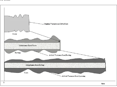
Figure 4 [40] below, explains the above concept using an example of density profiles of a sliver and the resulting roving and yarn in three successive processing stages. We can observe that at each stage the input variances of the previous processes i.e., the pre-existing variances in the process sums up with the variance component generated from that process itself and also the variance from the external causes which are not associated with the machineries. In order to analyze these variances the new dynamic process control system can be used.
Figure 4: Schematic Diagram of Inheritance of Variance from Previous
Process Stages
4.3.2 Methods of Achieving Variance Tolerancing
As mentioned earlier, Suh and Koo [4, 5] developed a novel method for achieving the variance tolerancing and decomposition applicable to fiber and yarn. They illustrated the process by the specific structure of the response variable Y as follows:
Let a textile product characteristic, Y, be
Y = g (X1... Xm\ h), m ≤ n, --- (13)
where g is a geometrical, probabilistic and structural model, x1, …, xm are the intrinsic components and h a set of intercepts which may equal to zero. Since the intercepts are not necessary for predicting Var (Y), Equation (13) can be written as
Y* = g* (X1… Xm), m ≤ n.
where Y* is a simplified form of Y and g* a modified function of g reflecting only the effects of Var (Xi) without regard to E (Xi), i = 1, 2, .., m.
The geometrical, probabilistic and structural models are often structure specific in that they may take account of the number of structural elements or units which contribute to textile product characteristics. The number of structural units contributing to a given characteristic of a textile product is usually determined by the geometrical structure of the product. In addition, the intensity of aggregating the structural units to forma textile structure is to be called „degree of constraints‟.
Equation (13). The estimated variances are compared to variances calculated based on the actual data in order to verify the theoretical estimates.
Based on the variance tolerancing through a geometrical, probabilistic and structural model with intrinsic components, the variance of a textile product characteristic can be estimated in terms of the statistical distributions of the intrinsic components. This can facilitate the optimal selection of input materials, process conditions and prediction/ optimization of textile product characteristics without having to rely heavily on the existing structural relationships that are often inadequate for a variance tolerancing. If each of X1 is associated with independent errors or variances, the classical statistical tolerancing formula by Tukey [41] can be applied to the Equation (13) to give
= --- (14) The Equation (14) is used to predict the variance of response Y in terms of the variances of the intrinsic components within their tolerance ranges. The variance, of a textile product characteristic can be estimated from input variances of intrinsic components through variance tolerancing based on geometrical probability and structural model. The total variance of the textile product can be decomposed into the variance tolerance from intrinsic components and those from each process.
let the variance of the product characteristic Y be σy2 when Y is found to be out-of-control. If
the variance estimated from raw materials is within the set limits, the input material can be eliminated from the list of suspicious factors. Through a sequential elimination of the innocent factors and processes, it is possible to narrow down the list to one or two factors or processes. In order to complete the task, however, it is necessary to pinpoint the time and location as well as the mechanism, structural relationship through which the situation was realized. The time is added as a new dimension based on a continuous monitoring and measurement scheme.
4.4
Advantages obtained using Dynamic Quality Control Systems
The new Dynamic Quality Control System developed, replaces the traditional static process average and the static stationary control limits by a dynamic process average and the associated dynamic control limits. This system will provide process averages and control limits that reflect what happened in the prior process stages. Also, this dynamic control system is thus designed in such a way that it prevents unnecessary corrective actions, minimizes the impact when the out-of-control situation causes an irreversible damage and provides a useful control system for searching the root causes of the out-of-control situations. Here are a few advantages of the dynamic control chart over the traditional static control chart (Shewhart Control Chart):
process widening the control limits to such an extent where they have now become almost useless in reducing the variance of the process. Hence, the dynamic quality control system is designed in such a way that the control limits obtained are more accurate than the ordinary static control limits.
Using the forward-prediction equations, the root causes of the „out-of-control‟ situations cannot be determined precisely as the back tracking of the responsible factors and processing conditions which produced the specific „out-of-control‟ situation often leads to a disappointing guess work rather than an effective solution. But using structural equations which connect the interlinking stages in a continuous process help us in determining the accurate root causes of the „out-of-control‟ situations. Hence, the dynamic quality control system determines the actual and accurate root causes of the out of control situations on a daily basis. The use of a static target reference in a continuous, dynamic textile process causes
frequent false alarms when the changes in process averages originate from the prior process stages. In order to minimize the unnecessary corrective actions (false positives) use of dynamic and flexible control limits is mandatory. Also, to minimize the loss of production time, materials and profit, the dynamic quality control chart is a best fit.
Chapter 5
Development of Dynamic Control Chart
& Variance Tolerancing - Application
in Ring Spinning Process
A conceptual/theoretical frame for a dynamic quality/process control system is being developed. The key strategy is to estimate the output process averages and variances as functions of the input process averages and also the variances originating from the prior process stage.