Plug-in Hybrid Electric Vehicle Control Strategies Utilizing Multiple Peaking Power Sources

(1)

University of Windsor University of Windsor

Scholarship at UWindsor

Electronic Theses and Dissertations Theses, Dissertations, and Major Papers

2010

Plug-in Hybrid Electric Vehicle Control Strategies Utilizing Multiple

Peaking Power Sources

Kevin Martin University of Windsor

Follow this and additional works at: https://scholar.uwindsor.ca/etd

Recommended Citation Recommended Citation

Martin, Kevin, "Plug-in Hybrid Electric Vehicle Control Strategies Utilizing Multiple Peaking Power Sources" (2010). Electronic Theses and Dissertations. 198.

https://scholar.uwindsor.ca/etd/198

This online database contains the full-text of PhD dissertations and Masters’ theses of University of Windsor students from 1954 forward. These documents are made available for personal study and research purposes only, in accordance with the Canadian Copyright Act and the Creative Commons license—CC BY-NC-ND (Attribution, Non-Commercial, No Derivative Works). Under this license, works must always be attributed to the copyright holder (original author), cannot be used for any commercial purposes, and may not be altered. Any other use would require the permission of the copyright holder. Students may inquire about withdrawing their dissertation and/or thesis from this database. For additional inquiries, please contact the repository administrator via email

(2)

PLUG-IN HYBRID ELECTRIC VEHICLE CONTROL STRATEGIES UTILIZING MULTIPLE PEAKING POWER SOURCES

By

KEVIN J. MARTIN

A Thesis

Submitted to the Faculty of Graduate Studies

through Mechanical, Automotive and Materials Engineering

in Partial Fulfillment of the Requirements for

the Degree of Master of Applied Science at the

University of Windsor

Windsor, Ontario, Canada

2010

(3)

PLUG-IN HYBRID ELECTRIC VEHICLE CONTROL STRATEGIES UTILIZING MULTIPLE PEAKING POWER SOURCES

By

KEVIN J. MARTIN

APPROVED BY:

___________________________________

N. Kar

Department of Electrical and Computer Engineering

___________________________________

J. Johrendt

Department of Mechanical, Automotive and Materials Engineering

___________________________________

B. Minaker, Advisor

___________________________________

A. Fartaj, Chair of Defense

(4)

Author’s Declaration of Originality

I hereby certify that I am the sole author of this thesis and that no part of this thesis has

been published or submitted for publication.

I certify that, to the best of my knowledge, my thesis does not infringe upon anyone’s

copyright nor violate any proprietary rights and that any ideas, techniques, quotations, or

any other material from the work of other people included in my thesis, published or

otherwise, are fully acknowledged in accordance with the standard referencing practices.

Furthermore, to the extent that I have included copyrighted material that surpasses the

bounds of fair dealing within the meaning of the Canada Copyright Act, I certify that I

have obtained a written permission from the copyright owner(s) to include such

material(s) in my thesis and have included copies of such copyright clearances to my

appendix.

I declare that this is a true copy of my thesis, including any final revisions, as approved

by my thesis committee and the Graduate Studies office, and that this thesis has not been

(5)

iv

Abstract

Conventional automobiles operate with the use of internal combustion engines (ICEs)

which run on fossil fuels as a source of energy. However, the conventional ICE provides

poor fuel economy, as well as producing air pollutants. A Plug-in Hybrid Electric

Vehicle (PHEV) has the potential to run solely on free energy with zero emissions as

long as it operates within its all electric range. Active control techniques must be used in

order to ensure optimum efficiency of the PHEV once the ICE is operated.

The objective of the proposed research is to create a control strategy utilizing batteries as

well as ultracapacitors suitable for a PHEV configuration. The control strategy will be

evaluated through numerical models under several driving cycles as well as emergency

maneuvers in order to ensure its effectiveness at reducing fuel consumption and

(6)

(7)

vi

Acknowledgements

I would like to first of all thank Dr. Bruce Minaker for the post Iron Ring ceremony

conversation that would eventually lead to my decision to begin my Masters under his

supervision. He permitted my ideas to wander freely and allowed me to discover a path

for myself, deepening my independence as a researcher and as an engineer.

It was a pleasure to work in the Vehicle Dynamics and Control Research group, where

creative thoughts and inspiration could be found everywhere. Specifically, I would like

to thank Dr. Rob Rieveley for all of his assistance, guidance and patience with me. I

would also like to thank my colleagues, Hart Honickman and Mike Johnston, for their

knowledge and easygoing personalities, which made the last two years very enjoyable in

110C.

I was also very fortunate to receive support from the AUTO21 Network of Centres of

Excellence and would like to extend my thanks to my fellow researchers at the University

(8)

vii

List of Tables

Table 3.1: Pure Slip Magic Formula ... 27

Table 3.2: Stock Chrysler Pacifica Parameters ... 32

Table 3.3: ERS Acceleration... 34

Table 3.4: ERS Braking ... 35

Table 3.5: ERS Highway Fuel Consumption ... 36

Table 3.6: ERS City Fuel Consumption ... 37

Table 4.1: UDDS Drive Cycle Characteristics ... 40

Table 4.2: ERS-UDDS Performance ... 41

Table 4.3: HWFET Drive Cycle Characteristics ... 42

Table 4.4: ERS-HWFET Performance ... 44

Table 4.5: US06 Drive Cycle Characteristics ... 45

Table 4.6: ERS-US06 Performance ... 47

Table 4.7: SC03 Drive Cycle Characteristics ... 48

Table 4.8: ERS-SC03 Performance ... 50

Table 4.9: NYCC Drive Cycle Characteristics ... 51

Table 4.10: ERS-NYCC Performance ... 53

Table 5.1: ERS EV Acceleration ... 64

Table 6.1: PPS Control Logic ... 83

(14)

xiii

List of Figures

Figure 2.1: Longitudinal Vehicle Force Depiction ... 5

Figure 2.2: Driveline Components ... 6

Figure 2.3: Longitudinal Tire Behaviour ... 8

Figure 2.4: Steady-State Equivalent Battery Circuit... 10

Figure 2.5: Randles Equivalent Battery Circuit ... 11

Figure 2.6: Ultracapacitor Equivalent Circuit ... 12

Figure 2.7: Motor Type Comparison Chart ... 14

Figure 2.8: All Electric Range vs. Blend Mode ... 18

Figure 2.9: Hybrid Energy Storage Operation ... 20

Figure 2.10: Urban Dynamometer Driving Schedule ... 22

Figure 3.1: Longitudinal Vehicle Dynamics Model ... 24

Figure 3.2: Behaviour of Magic Formula Tire Model ... 28

Figure 3.3: Equivalent Role Stiffness Model ... 29

Figure 3.4: ERS Acceleration ... 33

Figure 3.5: ERS Braking ... 34

Figure 3.6: ERS Highway Fuel Consumption ... 36

Figure 3.7: ERS City Fuel Consumption ... 37

Figure 4.1: ERS-UDDS Velocity Profile ... 40

Figure 4.2: ERS-UDDS Engine Trace and Fuel Consumption... 41

(15)

List of Figures xiv

Figure 4.4: ERS-HWFET Engine Trace and Fuel Consumption ... 43

Figure 4.5: ERS-US06 Velocity Profile... 46

Figure 4.6: ERS-US06 Engine Trace and Fuel Consumption ... 46

Figure 4.7: ERS-SC03 Velocity Profile ... 49

Figure 4.8: ERS-SC03 Engine Trace and Fuel Consumption... 49

Figure 4.9: ERS-NYCC Velocity Profile... 52

Figure 4.10: ERS-NYCC Engine Trace and Fuel Consumption ... 52

Figure 5.1: Hybrid Electric Vehicle Configuration ... 56

Figure 5.2: Quasi-static Energy Flow Simulator ... 57

Figure 5.3: 35Ah All Electric Range Simulation ... 58

Figure 5.4: Charge Resistance ... 59

Figure 5.5: Discharge Resistance ... 59

Figure 5.6: Open Circuit Voltage... 59

Figure 5.7: Motor-Generator Efficiency Contour ... 62

Figure 5.8: ERS EV Acceleration ... 63

Figure 6.1: Vehicle Control Systems ... 65

Figure 6.2: Varying Speed Constant Throttle ... 67

Figure 6.3: Constant Speed Varying Throttle ... 68

Figure 6.4: Integrated Hybrid Control Engine Trace ... 69

Figure 6.5: Integrated Hybrid Control Electric Motor Torque ... 69

Figure 6.6: Engine On-Off Control ... 70

Figure 6.7: Free Body Diagram of a Vehicle under Braking ... 71

Figure 6.8: Ideal Braking Force Distribution ... 73

Figure 6.9: Directional Instability due to Rear Wheel Lockup ... 74

Figure 6.10: Braking Process Analysis ... 76

Figure 6.11: Regenerative Braking Optimization Process ... 78

(16)

Figure 6.13: Regenerative Braking On-Off 0.5g ... 79

Figure 6.14: Regenerative Braking On-Off 0.7g ... 80

Figure 6.15: Optimal Regenerative Braking ... 81

Figure 6.16: Battery and Ultracapacitor Currents with a Step Current ... 83

Figure 6.17: Regenerative Braking with Battery Energy Source ... 84

Figure 6.18: Regenerative Braking with Hybrid Power Source ... 85

Figure 6.19: Hybrid Power Source Power Split... 85

Figure 6.20: Low Speed Ultracapacitor Recharge ... 86

Figure 6.21: Optimal PPS Control Low Power Demand ... 87

Figure 6.22: Optimal PPS Control High Power Demand ... 87

Figure 7.1: ERS-UDDS EV State of Charge ... 90

Figure 7.2: ERS-UDDS EV Currents ... 91

Figure 7.3: ERS-HWFET EV State of Charge ... 92

Figure 7.4: ERS-HWFET EV Currents ... 93

Figure 7.5: ERS-US06 EV Velocity Profile ... 94

Figure 7.6: ERS-US06 EV State of Charge ... 94

Figure 7.7: ERS-US06 EV Currents ... 95

Figure 7.8: ERS-SC03 EV State of Charge ... 96

Figure 7.9: ERS-SC03 EV Currents ... 96

Figure 7.10: ERS-NYCC EV State of Charge ... 97

Figure 7.11: ERS-NYCC EV Currents ... 98

Figure 7.12: ERS-UDDS Blend Mode State of Charge ... 99

Figure 7.13: ERS-HWFET Blend Mode State of Charge ... 100

Figure 7.14: ERS-HWFET Blend Mode EM Torque ... 101

Figure 7.15: ERS-HWFET Blend Mode ICE Torque ... 101

Figure 7.16: ERS-US06 Blend Mode State of Charge ... 102

(17)

List of Figures xvi

Figure 7.18: ERS-US06 Blend Mode ICE Torque ... 104

Figure 7.19: ERS-SC03 Blend Mode State of Charge ... 105

Figure 7.20: ERS-SC03 Blend Mode EM Torque ... 106

Figure 7.21: ERS-SC03 Blend Mode ICE Torque... 106

(18)

xvii

List of Notation

The notation throughout this work is used to denote mathematical types. The notations

for specific entities are listed below

Label Description

AER All electric range

BLDC Brushless direct current

C Capacitance

Cdl Double-layer capacitance

Cuc Ultracapacitor capacitance

CD Charge depleting

CS Charge sustaining

DOD Depth of discharge

ERS Equivalent roll stiffness

Fx,ij Longitudinal tire force

HEV Hybrid electric vehicle

HWFET Highway Fuel Economy Test

iL Leakage current

I2 Battery current

(19)

List of Notation xviii

Iq Quadrature stator current

Iuc Ultracapacitor current

ICE Internal combustion engine

Lm Magnetizing inductance

Lr Rotor inductance

Ls Stator inductance

NYCC New York City Cycle

p Poles

pb Brake pressure

PHEV Plug-in hybrid electric vehicle

PPS Peaking power source

Q0 Nominal battery capacity

Quc Ultracapacitor charge

r Wheel radius

re Effective wheel radius

Rct Charge-transfer resistance

Rd Diffusion resistance

Rin Internal resistance

Ro Ohmic resistance

Ruc Ultracapacitor internal resistance

SC03 Speed Correction 03

SOC State of charge

SR Slip ratio

Ud Direct voltage component

(20)

Uo Non-ohmic overpotential

Uoc Open-circuit voltage

Uq Quadrature voltage component

UDDS Urban Dynamometer Driving Schedule

US06 Supplemental Federal Test Procedure

Vc Ultracapacitor terminal voltage

Longitudinal displacement

Longitudinal velocity

Longitudinal acceleration

Lateral displacement

Lateral velocity

Lateral acceleration

ηc Charge efficiency

ηd Discharge efficiency

Roll rate

Roll acceleration

Yaw rate

Yaw acceleration

φd Direct stator resolved rotor flux

φq Quadrature stator resolved rotor flux

ωr Rotor frequency

ωv Stator voltage frequency

Rotational wheel velocity

(21)

1

Chapter 1

1 Introduction

The internal combustion engine has been the most prominent propulsion system used for

transportation purposes throughout the last century. The depletion of fossil fuel resources

and the rise in emissions has resulted in a need for more sustainable transportation

methods. As modern society continues to grow, so does the need for an increasing

number of vehicles for transportation. Trends predict that the fossil fuels located under

the earth’s surface are at risk of being entirely consumed in the near future. Hybrid

electric vehicles (HEVs) offer superior fuel economy and are a logical step in the

direction towards zero emissions vehicles. This chapter offers a brief history of hybrid

electric vehicles and the motivation behind such research.

1.1 Electrification of Vehicles

All current production vehicles rely on the combustion of fossil fuels as a means of

transforming chemical energy to mechanical energy through the use of an internal

combustion engine. The combustion of fossil fuels results in the production of nitrogen

oxides, carbon monoxides and unburned hydrocarbons, all considered toxins when found

in air. The production of gases such as carbon dioxide and methane also contribute to

global warming. If the use of fossil fuels continues on its current trend, the world’s fossil

fuel resources will be completely depleted by approximately 2038 [12].

The concept of HEVs was established in the late 1800s, although the use of the electric

(22)

provide sufficient amounts. Regenerative braking was also invented around this time,

providing a means for recuperating the vehicle’s kinetic energy in order to recharge the

peaking power source. The complexity of the advancements in the powertrain systems

were seen as troublesome and not worth the effort, considering the proven reliability of

the IC engine.

The need for reduced emissions and fuel consumption prompted the return of the HEV.

Improvements in battery technology and computation power allowed for complex hybrid

vehicle drivetrain control. Of utmost importance is the integrated hybrid control, which

modulates the internal combustion engine and electric motor. The desired goal of such a

control is to achieve minimal fuel consumption while maximizing regenerative

capabilities of the braking system.

Implementation and testing of integrated hybrid control can become very costly. The

advancements in computation power have allowed for vehicle simulation techniques to

be developed in order to safely and accurately model vehicle systems for fractions of the

costs of real world tests [7].

1.2 Research Outline

The goals of this research are to develop a plug-in hybrid electric vehicle model, simulate

real world drive cycles, and analyze the effect of the integrated hybrid control algorithms

when multiple peaking power sources are incorporated in the vehicle model.

The first objective of the research is to develop and validate a highly flexible hybrid

vehicle dynamics model. The flexibility is determined through the number of hybrid

vehicle configurations which can be achieved in the model and the validation is

established through comparison to specifications given by the manufacturer.

The second objective of the research is to implement hybrid controls to optimize the

(23)

Introduction 3

significance are the integrated hybrid drivetrain control, regenerative braking control, and

the peaking power source control.

Finally, the effect of the developed hybrid controls during real world drive cycles will be

evaluated.

1.3 Thesis Structure

This thesis consists of eight chapters and two appendices. In Chapter 1, the social and

environmental effects are introduced, providing the motivation for the research. In

Chapter 2, the relevant literature regarding existing technology and innovation are

discussed. In Chapter 3, vehicle dynamics modeling is established. This chapter mainly

includes the applicable equations of motion and longitudinal vehicle dynamics behaviour.

In Chapter 4, the drive cycles of interest are evaluated in terms of distance, velocity,

acceleration, energy and power. In Chapter 5, plug-in hybrid electric vehicle control

strategies are developed. The differences between all electric, charge sustaining and

blend modes are described. In Chapter 6, hybrid electric drivetrain components are

introduced. The discussion includes modeling of the electric components and their

selection for such an application. In Chapter 7, the results of the numerical simulations

are provided. Validations of the hybrid vehicle dynamics model and drive cycle

implementation are established. Finally, in Chapter 8, implications of the results in

(24)

4

Chapter 2

2 Literature Review

The addition of electrical propulsion components to a conventional vehicle structure

allows the vehicle to run potentially with zero emissions and higher efficiency. The

complexity of the hybrid electric vehicle drivetrain requires extensive design and

development that can be extremely costly at the empirical level. Existing vehicle

dynamics models, drivetrain models, and non-linear tire models can be used in

conjunction with battery, ultracapacitor and electric motor models in order to develop

simulation software for hybrid electric vehicles suitable for evaluating multiple hybrid

configurations and control. Each subsystem may contain their own control, while the

interaction of the subsystems may also be controlled through some hierarchy of control

schemes. This chapter will focus on the state of the art for the development of such a

hybrid electric vehicle simulation model.

2.1 Vehicle Dynamics and Simulation

When modeling a vehicle, a fixed axis system with its origin at the centre of mass of the

vehicle body is used in order to ensure constant inertial properties. The forward or

longitudinal direction of the vehicle is labeled the x-axis, the right or lateral direction of

the vehicle is labeled the y-axis, and the downward or vertical direction is labeled the

z-axis. Rotation of the vehicle body about the longitudinal axis is known as roll, about the

lateral axis is known as pitch, and about the vertical axis is known as yaw. The rotation

(25)

Literature Review 5

Therefore, most vehicle models contain ten degrees of freedom for the vehicle body and

wheels. The solution of ten second order differential equations could prove to be

challenging; however, with the use of modern numerical mathematics software, this can

be done quite easily. Most commercially available vehicle simulation software contains

many more degrees of freedom within their models. In order to evaluate preliminary

design ideas, the vehicle systems may be simplified and analyzed in particular directions

separately with sufficient accuracy.

2.1.1Longitudinal Vehicle Dynamics

Modeling a vehicle in the longitudinal direction is typically done for acceleration and

braking purposes. The vehicle is modeled as a single rigid body, and all lateral effects

are ignored. Vertical loads at both the front and rear tires represent both the left and right

sides of the vehicle lumped as single loads. Figure 2.1 below displays all of the forces

acting on the simplified longitudinal vehicle dynamics model.

Figure 2.1: Longitudinal Vehicle Force Depiction

Rolling resistance and aerodynamic drag act against the vehicle body and are modeled as

functions of vehicle velocity. The application of Newton’s second law on the centre of

mass results in:

(26)

The traction force provided by the propulsion unit is labeled Ftraction and the force required

to overcome hill climbing is labeled Fgrade. The grade force is a result of the vehicle

weight acting in the longitudinal direction during inclination. This vehicle model is

useful for gear optimization, engine selection, fuel consumption and some basic

performance estimations [24] [12] [17] [21] [16]. The user must understand the

limitations of such a model due to the large number of simplifications and assumptions

made. In terms of numerical computation, the model can be simulated easily once it has

been arranged into a first order form.

2.1.2Driveline Dynamics

To develop the traction force in the longitudinal model, an analysis of the driveline must

be completed. The driveline consists of a propulsion unit, clutch, gearbox, differential,

driveshaft, and wheels as illustrated in Figure 2.2.

Figure 2.2: Driveline Components

The propulsion unit is typically an internal combustion engine with varying degrees of

model complexity. The most common ICE model is completed empirically using

dynamometer testing results for varying throttle positions where spark advance, exhaust

gas recirculation, air to fuel ratio, and emissions are considered pre-calibrated control

variables [24] [21] [9]. Alternatively, the throttle can be modeled as a variable nozzle

and the engine modeled as a pump with particular cylinder volume, rotational speed and

volumetric efficiency [39] [4]. Propulsion unit power will be the limiting factor in

(27)

The clutch is used in order to allow the vehicle to come to rest without stalling the engine

and is typically modeled as a power loss of the transmission [24] [21]. The second

fraction of the transmission model is the gear box, which selects the appropriate gear for

a given vehicle speed. The gear box is typically designed to either have a geometric or

progressive gear ratio [17] [24].

The differential and driveshafts are characteristically modeled as lumped masses with

constant rotational inertia properties classically added to the effective mass of the vehicle.

Losses in either the differential or driveshafts may be included in the losses of the

transmission. The vehicle wheel is a much more complex component in the driveline and

will be discussed in the subsequent section.

2.1.3Pneumatic Tire Modeling

The forces created to accelerate, brake, and corner a vehicle occur at the road-wheel

interface. The vehicle’s motion depends completely on these forces and therefore creates

a major importance on the accuracy of the tire model. The major difficulty in modeling

tires is their non-linear behaviour in both longitudinal and lateral directions. Once the

throttle is pressed, the wheel starts to slip slightly, which results in a differential speed

between the wheel’s spin speed and the ground speed, resulting in the generation of a

longitudinal force. The longitudinal force generated is a function of slip ratio and vertical

(28)

Figure 2.3: Longitudinal Tire Behaviour

In order to calculate wheel slip, the tire contact velocity is approximated by the rotational

speed of the wheel and the effective tire radius. The relationship for longitudinal slip

ratio is defined as:

(2.2)

As the tire accelerates, in either direction, it deforms at the road-wheel interface, creating

a compressed zone and a stretched zone. The unloading of the tire does not occur in the

same manner as the loading of the tire, resulting in a hysteresis effect. This hysteresis

effect results in what is known as rolling resistance, which opposes the motion of the

wheel [16].

To accurately simulate vehicle motion, the tire model must encompass longitudinal slip,

lateral slip and the aligning moment. Many empirical tire models exist, though the

preferred tire model is the Pacejka Magic Formula. It is a notable improvement from the

Calspan model, though the major drawbacks of the formula remain the lack of tire data

(29)

2.2 Hybrid Electric Drivelines

The electric propulsion system of a hybrid vehicle introduces several new components to

the vehicle structure. Traction is generated through the use of one or more electric

motors powered by batteries, ultracapacitors or a generator unit coupled to the IC engine.

Modeling of such components may be difficult due to their non-linearities and state

dependent variables. Each subsystem must be modeled accurately and independently

before being integrated.

2.2.1Batteries

Batteries are devices that convert chemical energy into electrical energy. They are

typically a reversible energy storage system; therefore, they can be recharged through the

reverse chemical process. The requirements for HEV applications include: high specific

power, high specific energy, long calendar and cycle life, low initial and replacement

costs, high reliability, and high robustness.

Classically, specific energy is the first parameter of concern, as this will affect the range

of the vehicle. Power density is ranked next in terms of importance, as it will affect the

vehicle’s performance under acceleration and braking. Achieving both high energy

density and power density is possible, although it comes at increased costs. Battery

manufacturers typically specify the coulometric capacity of their batteries. The

coulometric capacity is defined as the number of ampere-hours (Ah) gained while

discharging the battery at a fixed current rate until a off voltage is achieved. The

cut-off voltage is the minimum allowable voltage, which is achieved at zero state of charge.

The state of charge, SOC, of the battery is the ratio of the remaining capacity to the fully

charged capacity of the battery. A fully charged battery has a SOC of 1, and a fully

discharged battery has a SOC of 0. The SOC can be monitored accurately through a

(30)

shows the relationship between current, nominal battery capacity (Q0) and state of charge.

To improve the accuracy of the model, the coulombic efficiency ‘ηc’ may also be

included.

(2.3)

Battery models vary in complexity; the more accuracy required the more complex the

model. The most basic of battery models consists of an open-circuit voltage source in

series with an internal resistance [21] [29].

Figure 2.4: Steady-State Equivalent Battery Circuit

The application of Kirchhoff’s voltage law for the equivalent circuit yields:

(2.4)

In this model, the open circuit voltage varies with the SOC. The internal resistance is a

combination of three different effects. The first is the ohmic resistance (Ro), the second

is the charge-transfer resistance (Rct), and the third is the diffusion resistance (Rd). The

major drawback of this model is that the resistances do not depend on current. The

processes involved are highly non-linear; therefore, models have been developed where

fitting techniques are used to interpret results from constant-current tests. Modifications

to the original model can be made to include effects of SOC and discharge current.

(31)

The constants κ1 and κ2 create a linear relationship between battery state of charge and

open circuit voltage, while the constants κ3 and κ4 vary the battery model for charging

and discharging events.

Modeling dynamic effects of a battery requires a more sophisticated model. There are

several different models that may be used; of these, the most common is the Randles

model [21] [8].

Figure 2.5: Randles Equivalent Battery Circuit

The Randles model includes a double-layer capacitor to reproduce capacitive effects of

the charge accumulation/separation that occur at the interface of the electrodes and the

electrolyte. Applying Kirchhoff’s voltage law once again for the new battery model

results in:

(2.6)

(2.7)

Often this model is altered to include several different effects, such as self-discharge,

occurring within the battery. The resistances may be written as functions of discharge

current to include more of the nonlinear effects. The most precise battery models include

(32)

effects [8] [15] [4] [39]. Batteries can also be modeled through fitting methods and

tabular data from experimental discharge and charging events.

2.2.2Ultracapacitors

Ultracapacitors are devices which store energy in the electric field of an electrochemical

double layer. They typically have a substantially higher specific power than batteries but

the tradeoff is that their specific energy is substantially lower. Ultracapacitors are useful

for applications such as acceleration and hill climbing [12].

Ultracapacitors differ from regular capacitors in material as well as physical process. The

energy is stored by the charge separation taking place in the layers that separate the

electrolyte and the electrodes. A separator is used to insulate the electrodes as well as to

store and immobilize the liquid electrolyte.

An equivalent circuit of an ultracapacitor can be derived for physical modeling. The

simplest model consists of a capacitor in series with a resistor.

Figure 2.6: Ultracapacitor Equivalent Circuit

The application of Kirchhoff’s voltage law results in:

(2.8)

(33)

Dynamic modeling of ultracapacitors also contains modifications similar to those from

the battery models, though the basic equivalent circuit is seen as more accurate in

ultracapacitors [21].

2.2.3Electric Motors

In electric and hybrid electric vehicles the electric motor provides a traction force through

a transmission and the driven wheels. The motor is usually reversible, allowing it to

convert electrical power from the batteries into mechanical power to drive the vehicle,

but also to convert mechanical power back into electrical power to recharge the batteries.

The latter of the two modes is known as generator mode, which occurs during the process

of regenerative braking. Desired characteristics of a traction motor are high efficiency,

low cost, high specific power, good controllability, fault tolerance, low noise, and

uniformity of operation.

Several different types of electric motors exist, and they can be organized into two main

categories: commutator motors and commutatorless motors. Direct current (DC) motors

are categorized as commutator motors as they contain commutators and brushes.

Alternating current (AC) motors such as induction and switched reluctance motors are

categorized as commutatorless. Commutatorless motors provide higher efficiency,

higher power density and lower operating cost, which are all important aspects to the

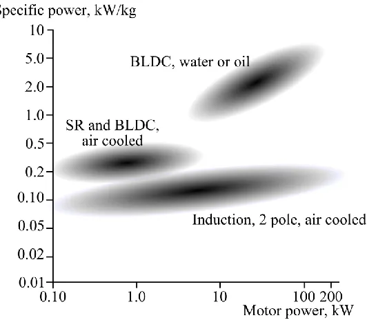
design of a HEV. This work will focus on the use of induction motors. Figure 2.4

shows the specific power of different types of electric motors suitable for traction motors

(34)

Figure 2.7: Motor Type Comparison Chart

Induction motors require an AC power source, usually supplied by an inverter with a DC

source. Induction motors are modeled using a two-phase reference frame. The reference

frame consists of a direct axis labeled‘d’, and a quadrature axis labeled ‘q’. The most

convenient reference frame is the synchronous reference frame which rotates at the

frequency of the magnetic field developed in the stator. Electrical circuit analysis of the

stator can be calculated using Kirchhoff’s voltage law.

(2.10)

(35)

The equations describing the state of the rotor are:

(2.12)

(2.13)

(2.14)

The d-q axis stator currents are Id(t) and Iq(t), the d-q axis stator voltages are Ud(t) and

Uq(t), and the d-q axis stator resolved rotor fluxes are φd(t) and φq(t). The stator resolved

rotor and stator inductances are Lr and Ls, the stator resolved rotor and stator resistances

are Rr and Rs, and the magnetizing inductance is Lm. The frequency of the stator voltage

is represented by ωv(t), and the frequency of the magnetic field induced in the rotor is

given by the number of poles, p, multiplied by the rotor speed, ωr(t) [21] [20] [12] [13].

The magnetic field induces a torque on the rotor which can be found through an energy

balance. Stator voltage components and the AC frequency are set by the electronic

frequency converter. The main power electronics of the motor system is the inverter,

which converts the DC supply voltage to a variable frequency three phase AC source.

The losses of the system come from ohmic resistance, slip and controller efficiency. In

order to solve the equations of the system, the stator voltages and frequency must be

known from the control strategy. Equations 2.10-2.13 can then be integrated to solve for

the currents and fluxes of the d-q reference frame. A common control strategy is to

impose zero d-axis voltage and to modulate the q-axis voltage as a function of supply

voltage [21]. Alternatively, empirical modeling of the motor may be conducted to

develop an efficiency contour for a given motor once the motor controller has been

(36)

2.3 Plug-in Hybrid Electric Vehicle Control

The integration of conventional vehicle components with electric propulsion components

results in a vast number of potential hybrid electric configurations. A series hybrid is

characterized by a configuration in which the electric motor alone provides the traction

force for the vehicle. The power can be provided by either the battery or by a generator

driven by an ICE. Alternatively, a parallel hybrid vehicle is characterized by a

configuration in which either the electric motor or the internal combustion engine can

provide the traction force for the vehicle. Several other configurations exist, though they

are typically a combination of the series and parallel types [19] [7] [14] [25].

As the complexity of the vehicle configuration is increased, so are the demands for

control. Each vehicle component must have its own control, though the interaction of the

various subsystems must also be controlled. In order to achieve the optimal result, three

main types of subsystem interaction control are required: integrated hybrid control,

regenerative braking control, and multiple power source control.

2.3.1Integrated Hybrid Control Strategies

The goal of integrated HEV control is to determine the optimal power split at each instant

of time that minimizes the total fuel consumption of the vehicle [38] [19]. Classical

hybrid electric vehicles charged their batteries solely from fuel transformed through the

internal combustion engine and generator; therefore, they typically hold the SOC at some

constant value where the battery efficiency is greatest. In contrast, plug-in hybrid electric

vehicles recharge their batteries at the end of a driving event, allowing the battery to run

through a range of depletion levels. The energy gained during plug-in charging can be

taken from natural or free resources, where zero emissions are produced. As a result, it is

desired that the initial battery state be fully charged and that the final state be completely

(37)

from the battery during the driving event [26]. In order for the battery to achieve zero

SOC at the end of the driving event, two strategies are available; all electric control and

blend mode control.

2.3.1.1 All Electric Range Control

The purpose of the All Electric Range Control (AER) is to allow the vehicle to utilize its

entire battery range before switching to fuel for energy [26] [45]. If the vehicle has an all

electric range of 40 miles and travels 20 miles daily, the vehicle can be recharged at the

end of each day and never consume any fuel, acting as an electric vehicle. Once the SOC

reaches the minimum threshold, charge sustaining mode (CS) is automatically initiated.

Charge sustaining mode holds the battery state of charge near constant to ensure the

battery does not reach dangerously low levels, which will affect battery life. For plug-in

hybrid electric vehicles with large AERs, this control strategy is the most fuel efficient.

For PHEVs with small AERs, a charge depleting mode such as blend mode control is

most fuel efficient [26]. The battery state of charge for all electric control can be seen in

Figure 2.8 where B represents EV mode operation and A represents CS mode operation.

2.3.1.2 Blend Mode Control

Blend mode control uses both the IC engine and the electric motor until the SOC of the

battery reaches the minimum threshold. Given that fuel and battery split the energy

demand, the blend mode reaches the CS mode much later than AER control. The engine

is only operated when it can perform within its optimal efficiency range, but is also

dependent on the battery SOC, throttle position and prior knowledge of trip distance [26]

[45] [25]. The battery state of charge throughout blend mode operation is seen in Figure

(38)

Figure 2.8: All Electric Range vs. Blend Mode

As the engine operates in a high efficiency range, the electric motor is used as a power

modulator [7]. The engine and motor can also be used for power assist purposes,

increasing acceleration performance or downscaling to save mass [41]. The integration

of the two subsystems results in a complex situation of control. Three types of blend

mode control exist: dynamic programming, intelligent control techniques such as fuzzy

logic, and optimal control [38] [19] [18]. All of these have been successfully

implemented, although optimal control tends to require information that is unknown for a

given driving event, such as SOC and total distance; therefore, optimal control may prove

too complex for practical use [19] [26] [10].

The selection of the control strategy and control type will be based strongly on the

topology of the vehicle as well as the performance index. The input variables must be

easily measurable and the control scheme must be robust and reliable [25] [19]. System

efficiencies of plug-in hybrid electric vehicles have been nearly doubled in test

(39)

2.3.2Regenerative Braking Systems

One of the most important features of a hybrid electric vehicle is the ability to recapture

significant amounts of energy during braking. Conventional braking systems dissipate

kinetic energy as heat through friction. Conversely, HEVs run the motor as a generator,

recharging the batteries and improving fuel efficiency and range [1] [12] [37] [44].

Regeneration is limited by the available capabilities of the traction motor and the battery

system. Due to the limitations of the batteries and motor, a friction braking system must

be used for emergency braking and bringing the vehicle to rest [48]. Hybrid control must

also be developed for the hybrid braking system. The purpose of the hybrid braking

control is to ensure maximum regenerative torque upon a braking request. As the

maximum regenerative torque is being provided, the controller must also modulate the

friction brakes to meet driver demand. Previous active safety systems such as anti-lock

braking (ABS), electronic braking force distribution (EBD), traction control (TC) and

electronic stability program (ESP) can all be incorporated into the hybrid braking

scheme. The control strategy must monitor the battery SOC, battery temperature, and

available motor torque in order to guarantee optimal braking [1] [37] [48].

2.3.3Multiple Peaking Power Sources

The use of traction batteries provides many advantages such as recuperation of energy

when braking, idling on electric power to avoid emissions, driving on electrical power in

specific cases where the IC engine has poor emissions, and decreased fuel consumption

[2] [42]. However, the battery is very rate sensitive and has limited power capabilities.

The introduction of a secondary power source to a hybrid vehicle can allow the system to

overcome some of the downfalls of lone energy storage. Limitations on drive range are a

(40)

a result of poor power density. The hybridization of ultracapacitors and batteries allows

compensation for the lower specific energy of the ultracapacitors and the lower specific

power of the batteries [12] [6] [49].

Figure 2.9: Hybrid Energy Storage Operation

Ultracapacitors have the ability to absorb high currents with high frequencies over nearly

endless cycles without performance deterioration, making them an ideal counterpart for

batteries, which can be extremely sensitive to large discharge and charge rates [6] [11]

[36]. Acceleration and regenerative braking tend to cause large currents which exceed

battery limitations.

The integration of ultracapacitors and batteries results in the need for a control strategy to

regulate their current demands. The ultracapacitor SOC is controlled based on vehicle

(41)

to ensure that maximum regenerative braking can be achieved even with high battery

SOC [36] [11]. The ideal case will allow the ultracapacitors to take full loads for short

pulses and not cause any sudden spikes in battery current. In other words, the

ultracapacitor handles the transients of the system, while the battery handles the majority

of the steady-state demand [3]. The addition of ultracapacitors to a battery energy

storage system can significantly improve power and vehicle range without any increase

on cost or vehicle mass [36].

2.4 Drive Cycles

To model the range and efficiency of a proposed HEV, it is important to have relevant

drive data for simulation purposes. Before driving data was available, constant velocity

tests were customary [12]. It is obvious that constant velocity tests would produce only

moderately accurate results as real driving scenarios would be ignored. Many

corporations have gone through the task of instrumenting fleets of vehicles in order to

develop real world driving data, also known as drive cycles. They are a useful tool for

comparative studies between HEVs, although their accuracy could be questioned. Drive

cycles allow for simulation in which the vehicle undergoes realistic driving patterns of

everyday use. The development of real world drive cycles has created a push towards

standardized hybrid electric vehicle fuel consumption calculations. The Society of

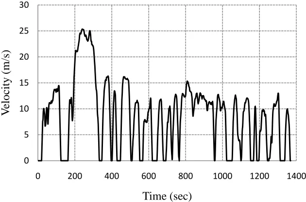
Automotive Engineers Journal J1711 sets forth a standard for evaluating HEV fuel

consumption under testing of four primary drive cycles: UDDS, HWFET, US06, and

(42)

Figure 2.10: Urban Dynamometer Driving Schedule

According to current federal test procedure standards, the vehicle must not miss the speed

trace by more than 2 mph (0.89 m/s) at any point in time [31]. Fuel displacement

benefits of PHEVs will also be influenced by the frequency of recharging events [30].

The availability of drive cycle data has created a large market of HEV simulations for

hybrid electric vehicle control optimization. Some preliminary results show a lack in

correlation between simulation and empirical testing. Suggestions have been made that

errors may be a result of unexpected engine on/off behaviour as a result of throttle

uncertainty [43] [28]. Driver aggressiveness, range and the exclusion of effects such as

thermal behaviour, component wear and weather conditions have also been linked to the

inaccuracies of the simulation results [34] [43]. Despite some early discrepancies, drive

cycles remain the main estimator of fuel economy and all electric range for plug-in

hybrid electric vehicles [46].

0 5 10 15 20 25 30

0 200 400 600 800 1000 1200 1400

V

elocity

(m/s)

(43)

23

Chapter 3

3 Vehicle Dynamics and Simulation

Vehicle dynamics may be analyzed in several different ways. Typically models are

developed for isolated analysis of a particular case. Vehicle models range in complexity

from a simple one degree of freedom model to extremely complicated multibody

systems. Although modeling of an entire vehicle and all of its subsystems would prove to

be the most accurate, the time consumption of such models is undesirable. The

development of a vehicle dynamics model must reduce the model complexity of the

entire system, be implemented in a common PC programming language, include

interactions of the subsystems of interest, and be only as accurate as necessary, saving

valuable computation time.

In order to model the full vehicle system, subsystems for the suspension, engine,

driveline, and chassis should also be incorporated. The inputs of the engine and driveline

subsystems will originate from driver demand as throttle and brake. The inputs of the

chassis and body subsystems will originate from the driver steer angle and road

geometry. The following sections will focus on the development of a vehicle dynamics

model for hybrid electric vehicle simulation purposes.

3.1 Longitudinal Vehicle Dynamics

The primary direction of interest when developing a vehicle dynamics model for HEV

applications is the forward or longitudinal direction. Classically, HEVs are modeled

(44)

effects are ignored due to low cornering speeds and vertical effects are ignored due to

assumed flat road geometry.

The vehicle is modeled as five masses; one lumped mass and four wheel masses. The

single lumped mass includes the mass of the body, engine, driveline, fuel, passengers,

and any other payload. It has a sole degree of freedom, translation in the longitudinal

direction. The four wheel masses are each assigned a degree of freedom, rotation about

the wheel center. A schematic of the longitudinal vehicle dynamics model can be seen in

Figure 3.1.

Figure 3.1: Longitudinal Vehicle Dynamics Model

The equations of motion of the system can be derived from Newton’s second law as:

(3.1)

(3.2)

The torque output from the engine through the drivetrain is labeled Tengine, the moment

created about the wheel centre due to rolling resistance is labeled Mrolling resistance, the

longitudinal contact patch friction force is labeled MFx, and the torque developed by the

braking system based on brake pedal position is labeled Tbrake. The wheel moment

equation is applied separately for each wheel in the model. The driveline is modeled

using classical modeling techniques discussed in Section 2.1.2 and the tire forces are

(45)

Vehicle Dynamics and Simulation 25

3.2 Tire Forces

The tire model is the single most important part in a vehicle dynamics model. It is

responsible for transferring forces from the vehicle to the road and vice versa. In order to

model a tire, first the tire characteristics must be estimated or obtained from experimental

tests. All tire compounds are different and therefore no model will be able to model all

tire behaviour.

Friction in the tire is generated through two main effects; adhesion and hysteresis.

Adhesion is a result of the molecular bonds generated between the exposed surface of

atoms of rubber and road material in the contact area, where as hysteresis is a result of a

difference in loading and unloading forces.

Tractive and lateral forces are a function of normal force, slip angle and slip ratio. Slip is

always present in the tire even with no tractive driving or braking forces. All forces

acting at the road tire interaction surface are assumed to occur at the centre of the contact

patch.

3.2.1Wheel Speed Stability

The slip ratio has alternate definitions under driving and braking conditions. Under

driving a slip ratio of one is defined as wheel spin and under braking a slip ratio of one is

defined as fully locked. Peak longitudinal forces occur at slip ratios of 0.15 to 0.3, slip

ratios smaller than those at peak values tend to converge, though larger values of slip tend

to diverge rapidly until torque is reduced [27].

The definition of slip ratio works well for forward velocities but has inherent problems

when low speeds and negative velocities are considered. It is desired to modify the

definition of slip ratio to contain all cases of acceleration and braking in all directions,

(46)

(3.3)

This correction has addressed the issue of negative velocities, though does not address the

singularity in wheel slip as the wheel speed approaches zero. The solution is to derive a

first order differential equation for longitudinal slip.

(3.4)

The solution found from Equation 3.4 results in oscillations at low vehicle speeds. To

eliminate these oscillations, a damping term which is only active at low speeds is

introduced.

(3.5)

The damping term is activated in the wheel speed equation at speeds lower than 0.15 m/s

where ζ is the damping coefficient, Cs is the longitudinal stiffness, and B is equivalent to

that found in Equation 3.4 and is experimentally determined (0<B<1). The sign of the

damping term must switch at each time step to ensure sufficient oscillation reduction in

the wheel speeds [32].

3.2.2The Magic Formula Tire Model

The function of the tire model is to establish the forces and moments occurring at the tire

road contact patch and resolve these to the wheel centers and hence into the vehicle

chassis. The forces needed for vehicle handling are: longitudinal tractive or braking

force, lateral cornering force, vertical normal force, and the aligning moment.

The tire model must continually receive information about the position, orientation, and

(47)

The Magic Formula Tire model was introduced by Bakker in 1986 and has seen

widespread acceptance in vehicle dynamics literature [5]. The Magic Formula relates

lateral force to slip angle, aligning moment to slip angle and longitudinal force to slip

ratio. Previously completed experiments show a high correlation between the Magic

Formula and actual data. The equations of the Magic Formula are summarized in Table

3.1.

General Formula Longitudinal Force

Table 3.1: Pure Slip Magic Formula

The value of Y(X) is either the lateral force, aligning moment, or longitudinal force. The

value of x is the corresponding input to the model, either slip angle or slip ratio. The

(48)

physical features such as conicity and ply steer and are related to the lateral and aligning

moment formulae. The peak factor, D, determines the upper limit of the transmissible

force. The shape factor, C, controls the stretching of the curve in the x direction and has

typical values of 1.3, 1.65 and 2.4 for lateral, longitudinal and aligning moment

respectively. The stiffness factor, B, is multiplied by C and D to create the slope at the

origin. The curve factor, E, effects the transition in the curve and the position of the peak

value. The coefficients b0 through b13 are listed in Appendix A. The resulting

longitudinal force versus slip ratio and normal load can be seen in Figure 3.2.

Figure 3.2: Behaviour of Magic Formula Tire Model

3.3 Equivalent Roll Stiffness Model

The Equivalent Roll Stiffness (ERS) model is developed from the lumped mass model by

treating the front and rear suspensions as rigid axles connected to the body by revolute

joints [5]. The model also includes yaw effects as a result of steer inputs from the driver.

The ERS model has been proven successful in implementation for variable torque

(49)

model results in eight degrees of freedom: longitudinal translation, lateral translation,

yaw rotation, roll rotation, and the four rotations of the wheels.

Figure 3.3: Equivalent Role Stiffness Model

Despite the minimum requirements of longitudinal vehicle dynamics isolation for HEV

applications, the Equivalent Roll Stiffness model allows for some expansion of the

desired simulations. The developed controls may now be tested for sensitivity in

cornering as well as emergency maneuvers through the ERS model. The resulting

equations of motion can be written according to Newton’s second law as [40] [27] [22]:

(3.6)

(3.7)

(3.8)

(3.9)

(3.10)

(50)

(3.12)

(3.13)

The estimation of the roll stiffness for the ERS model is done by separately analyzing the

roll stiffness, Ks, and roll damping, Cs, of the front and rear axle. The estimation of roll

damping is obtained by assuming equivalent linear damping and using the positions of

the dampers relative to the roll centers to calculate the required coefficients. The

estimation of the roll stiffness is done in a similar manner, although contributions of the

anti-roll bars must also be included. To further understand the developed ERS model,

examination of its subsystems will be conducted in the following sections.

3.3.1Driver Behaviour

The ERS driver model contains three control variables: throttle, brake and steer angle.

The throttle is a closed loop PID controller set for vehicle speed correction. A control

gain for driver aggressiveness may also be selected.

The steer angle can be calculated from a set of five different functions: no steer, steady

steer, double lane change, sinusoid, increasing sinusoid, or ramp. All steer functions

contain an initializing time delay and a final time delay [40].

3.3.2Powertrain and Driveline

The ERS powertrain is modeled as a quasi-static engine efficiency map with idle and

redline limitation parameters. The engine is coupled to a non-linear torque converter,

modeled by a fourth order polynomial, and an automatic transmission. The model allows

for flexible powertrain configurations including: front wheel drive, rear wheel drive, and

(51)

and driveline subsystem. Operating efficiency is calculated as a ratio of power out to fuel

power utilized. All engine thermal effects are neglected in the ERS model [40].

3.3.3Hydraulic Braking

The ERS model employs a classical hydraulic braking system to decelerate the vehicle.

The braking torque is generated through friction between the pads and rotors and is

modeled as [5]:

(3.14)

Where n is the number of friction surfaces, μb is the coefficient of friction between the

pads and the rotor, pb is the brake pressure, Ab is the brake piston area, and Rd is the

radius to the center of the pad. The brake pressure is modulated through a close looped

feedback controller set for speed correction. Thermal effects of the braking system are

neglected.

3.4 Simulation

Once the set of ordinary differential equations that represent the system have been

developed, the ODEs must then be rewritten into first order form for numerical

integration. The program chosen for the numerical integration of the vehicle model is

MATLAB®. MATLAB contains several ODE solvers suitable for systems of differential

equations. The ODE45 routine is an explicit Runge-Kutta (4,5) formula with moderate

accuracy requiring only the solution at the preceding time step, making it suitable for the

given vehicle model. Numerical stiffness may hinder simulation time of this solver if not

(52)

3.5 Validation Results

Preceding the hybridization of the ERS model, validity of the model must be established.

Due to the longitudinal nature of the simulations, the ERS model will be validated using

four primary tests: longitudinal acceleration, longitudinal braking, highway fuel

consumption, and city fuel consumption. The tests will be conducted using a model of a

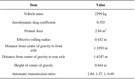
stock Chrysler Pacifica. The parameters of the Pacifica can be seen in Table 3.2.

Item Value

Vehicle mass 2299 kg

Aerodynamic drag coefficient 0.355

Frontal Area 2.84 m2

Effective rolling radius 0.432 m

Distance from center of gravity to front

axle 1.3293 m

Distance from center of gravity to rear axle 1.6247 m

Height of center of gravity 0.644 m

Automatic transmission ratios 2.84, 1.57, 1, 0.69

(53)

3.5.1Acceleration

To evaluate the accuracy of the ERS model, the stock Pacifica configuration will be

modeled and tested in a drag strip acceleration simulation. The results of the ERS

acceleration test are seen in Figure 3.4.

Figure 3.4: ERS Acceleration

Figure 3.4 shows the velocity and acceleration time history of the ERS drag strip

acceleration simulation. Close examination of the results shows transmission gear shifts

at 5 and 13.5 seconds. Table 3.3 lists the corresponding acceleration times for the

Pacifica from an empirical test. Correlation of the times from Table 3.3 to the times

found by the ERS model will prove validity in acceleration.

Acceleration Time (seconds) ERS Time (seconds)

Relative Error (%)

0-30 mph 3.1 3.18 2.54

0-40 mph 4.7 4.51 4.12

0-50 mph 6.8 6.59 3.13

(54)

0-70 mph 12.6 11.94 5.37

0-80 mph 16.4 16.47 0.42

0-90 mph 22.0 22.37 1.66

0-100 mph 29.6 31.68 6.78

Table 3.3: ERS Acceleration

The results from the ERS model show a correlation coefficient of 0.998. Relative errors

are calculated and found to be less than 10% during all operational speeds. The relative

errors are a result of many factors including: model inaccuracies, parameter estimations,

and lack of experimental data (i.e. temperature, wind conditions, road surface, etc.). The

correlation of the results with empirical test data has proven the ERS model valid in

acceleration.

3.5.2Braking

To evaluate the accuracy of the ERS model, the stock Pacifica configuration will be

modeled and tested in a braking simulation. The results of the ERS braking test are seen

in Figure 3.5.

Plug-in Hybrid Electric Vehicle Control Strategies Utilizing Multiple Peaking Power Sources

Scholarship at UWindsor

Scholarship at UWindsor

Plug-in Hybrid Electric Vehicle Control Strategies Utilizing Multiple

Plug-in Hybrid Electric Vehicle Control Strategies Utilizing Multiple

Peaking Power Sources

Peaking Power Sources

Author’s Declaration of Originality

Abstract

Acknowledgements

Table of Contents

List of Tables

List of Figures

List of Notation

Chapter 1

1 Introduction

1.1

Electrification of Vehicles

1.2

Research Outline

1.3

Thesis Structure

Chapter 2

2 Literature Review

2.1

Vehicle Dynamics and Simulation

2.2

Hybrid Electric Drivelines

2.3

Plug-in Hybrid Electric Vehicle Control

2.4

Drive Cycles

Chapter 3

3 Vehicle Dynamics and Simulation

3.1

Longitudinal Vehicle Dynamics

3.2

Tire Forces

3.3

Equivalent Roll Stiffness Model

3.4

Simulation

3.5

Validation Results