Mining High Utility Sequential Patterns from Uncertain Web Access Sequences using the PL-WAP

(1)

University of Windsor University of Windsor

Scholarship at UWindsor

Electronic Theses and Dissertations Theses, Dissertations, and Major Papers

2017

Mining High Utility Sequential Patterns from Uncertain Web

Access Sequences using the PL-WAP

Sravya Vangala University of Windsor

Follow this and additional works at: https://scholar.uwindsor.ca/etd

Recommended Citation Recommended Citation

Vangala, Sravya, "Mining High Utility Sequential Patterns from Uncertain Web Access Sequences using the PL-WAP" (2017). Electronic Theses and Dissertations. 6022.

https://scholar.uwindsor.ca/etd/6022

This online database contains the full-text of PhD dissertations and Masters’ theses of University of Windsor students from 1954 forward. These documents are made available for personal study and research purposes only, in accordance with the Canadian Copyright Act and the Creative Commons license—CC BY-NC-ND (Attribution, Non-Commercial, No Derivative Works). Under this license, works must always be attributed to the copyright holder (original author), cannot be used for any commercial purposes, and may not be altered. Any other use would require the permission of the copyright holder. Students may inquire about withdrawing their dissertation and/or thesis from this database. For additional inquiries, please contact the repository administrator via email

(2)

i

Mining High Utility Sequential Patterns from Uncertain

Web Access Sequences using the PL-WAP

By

Sravya Vangala

A Thesis

Submitted to the Faculty of Graduate Studies through the School of Computer Science

in Partial Fulfillment of the Requirements for the Degree of Master of Science at the

University of Windsor

Windsor, Ontario, Canada

2017

(3)

ii

Mining High Utility Sequential Patterns from Uncertain Web Access

Sequences using the PL-WAP

by

Sravya Vangala

APPROVED BY:

______________________________________________

S. Nkurunziza

Department of Mathematics and Statistics

______________________________________________

R. Gras

School of Computer Science

______________________________________________

C. I. Ezeife, Advisor School of Computer Science

(4)

iii

AUTHOR’S DECLARATION OF ORIGINALITY

I certify that I am the sole author of this thesis and that no part of this thesis has been published or submitted for publication.

I certify that, to the best of my knowledge, my thesis does not infringe upon anyone’s copyright nor violate any proprietary rights and that any ideas, techniqus, quotations, or any other material from the work of other people included in my thesis, published or otherwise, are fully acknowledged in accordance with the standard referencing practices. Furthermore, to the extent that I have included copyrighted material that surpasses the bounds of fair dealing within the meaning of the Canada Copyright Act, I certify that I have obtained a written permission from the copyright owner(s) to include such material(s) in my thesis and have included copies of such copyright clearances to my appendix.

(5)

iv

ABSTRACT

In general, the web access patterns are retrieved from the web access sequence databases using various sequential pattern algorithms such as GSP, WAP and PLWAP tree. However, these algorithms do not consider sequential data with quantity (internal utility) (e.g., the amount of the time spent by the user on a web page) and quality (external utility) (e.g., rating of a web page in a website) information. These algorithms also do not work on uncertain sequential items (e.g., purchased products) having probability (0, 1). Factoring in the utility and uncertainty of each sequence item provides more product information that can be beneficial in mining profitable patterns from company’s websites. For example, a customer can purchase a bottle of ink more frequently than a printer but the purchase of a single printer can yield more profit to the business owner than purchase of multiple bottles of ink. Most existing traditional uncertain sequential pattern algorithms such as U-Apriori, UF-Growth, and U-PLWAP do not include the utility measures. In U-PLWAP, the web sequences are derived from weblog data without including the time spent by the user and the webpages are not associated with any rating. By considering these two utilities, sometimes the items with lower existential probability can be more profitable to the website owner. In utility based traditional algorithms, the only algorithm related to both uncertain and high utility is PHUI-UP algorithm which considers the probability and utility as different entities and the retrieved patterns are not dependent with both due to two different thresholds, and it does not mine uncertain web access database sequences.

This thesis proposes the algorithm HUU-PLWAP miner for mining uncertain sequential patterns with internal and external utility information using PLWAP tree approach that cut down on several database scans of level-wise approaches. HUU-PLWAP uses uncertain internal utility values (derived from sequence uncertainty model) and the constant external utility values (predefined) to retrieve the high utility sequential patterns from uncertain web access sequence databases with the help of U-PLWAP methodology. Experiments show that HUU-PLWAP is at least 95% faster than U-PLWAP, and 75% faster than PHUI-UP algorithm.

(6)

v

DEDICATION

(7)

vi

ACKNOWLEDGEMENT

My sincere appreciation goes to my mentor Baba, grandparents MohanaRao & Sailaja, parents Sekhar & Bhargavi and in-laws Harinadhababu & Vasantha. Your perseverance and words of encouragement gave me the extra energy to see this work through.

I will be an ingrate without recognising the invaluable tutoring and supervision from Dr. Christie Ezeife. Your constructive criticism and advice always gave me the needed drive to complete this work. I like to thank Dr. C. I. Ezeife for continuous research assistantship positions.

Special thanks go to my external reader, Dr. Severien Nkurunziza, my internal reader, Dr. Robin Gras and the chair, Dr. Luis Rueda for accepting to be on my thesis committee. Your decision, despite your tight schedules, to help in reading the thesis and providing valuable input is highly appreciated.

(8)

vii

LIST OF TABLES

Table 1: Number and percentage of students regarding class obtained ...2

Table 2: Number of Students Regarding Class ...3

Table 3: Percentage of students...3

Table 4: A Sample Transaction Database ...4

Table 5: Weblog Sequence Database ...7

Table 6: A Traversal Path Database and Profit Table... 13

Table 7: Speeding Vehicle Records ... 17

Table 8: Number of possible worlds from the Speeding Vehicle records ... 17

Table 9: Example of a Relation with x-tuples ... 19

Table 10: Example of a relation with Attribute Uncertainty ... 20

Table 11: Certain vs. Uncertain Data ... 20

Table 12: Summary of the existing systems with their limitations ... 26

Table 13: Transaction database (Han et al., 2000) ... 32

Table 14: The FP-growth mining process (Han et al., 2000) ... 33

Table 15: Web Access Sequence Database ... 34

Table 16: A Sample database of web access sequences (Pei et al., 2000) ... 36

Table 17: The Web Access Sequence Database (Ezeife and Lu 2005) ... 38

Table 18 : Sample uncertain sequence (Kadri and Ezeife 2011) ... 43

Table 19: Transaction Database ... 46

Table 20: Quality Table... 46

Table 21: Uncertain Transaction database ... 51

Table 22: Examples of (a) sequence database (b) external utility (Ahmed et al., 2010) ... 55

Table 23: Candidate generation process for UL algorithm (Ahmed et al., 2010) ... 56

Table 24: Candidate generation process for US algorithm (Ahmed et al., 2010) ... 59

Table 25: A Single Sequence Database with Five Transactions ... 61

Table 26: Profit Table ... 61

Table 27: Uncertain Sequence Database from Windsor Star Website ... 72

Table 28: Corresponding possible worlds ... 74

Table 29 : UWASDB with Internal Utilities & Existential Probabilities ... 76

Table 30: Uncertain Web Access Sequence Database (UWASDB) with Probabilistic Internal Utilities .. 76

Table 31: Profit Table ... 77

Table 32: waswu values... 80

Table 33: The performance of HUU-PLWAP and PHUI-UP with different min WAS Threshold ... 86

Table 34: The performance of HUU-PLWAP and U-PLWAP with different min WAS Threshold ... 87

Table 35: Memory consumption of HUU-PLWAP, PHUI-UP with different min WAS Threshold ... 88

(11)

x

LIST OF FIGURES

Figure 1: Vertical Bitmap of items in database ...7

Figure 2: Lexicographic tree ...8

Figure 3: The S-step and I-Step procedures ...9

Figure 4: Constructed FP-Tree (Han et al., 2000) ... 32

Figure 5: Example of web access pattern tree (Pei et al., 2000) ... 37

Figure 6: The PLWAP tree with the header linkages (Ezeife and Lu 2005) ... 39

Figure 7: U-PLWAP Tree Constructed from the Example in the Table 18 ... 44

Figure 8: Transaction Database and Profit Table (Bakariya and Thakur 2015) ... 48

Figure 9: Transaction Table ... 49

Figure 10: Sample LQS Tree (Yin et al., 2012) ... 62

Figure 11: The HUU-PLWAP algorithm ... 66

Figure 12: The Frequent-1 Waswu algorithm ... 67

Figure 13: HUU-PLWAP -tree construction algorithm. ... 69

Figure 14: The Mine Algorithm ... 71

Figure 15 : The complete linked HUU-PLWAP tree ... 81

Figure 16: Comparing execution time of HUU-PLWAP & PHUI-UP with different min WAS Threshold . 87 Figure 17: Comparing execution time of HUU-PLWAP & U-PLWAP with different min WAS Threshold 87 Figure 18: Memory utilised for the HUU-PLWAP, PHUI-UP with different min WAS Threshold ... 88

(12)

1

1. INTRODUCTION

1.1. DATA MINING

Data mining refers to the knowledge discovery from data (KDD), the KDD process include (a) data selection (which retrieves from databases those target data, i.e., data relevant to the analysis task), (b) data pre-processing (which integrates target data from various sources and cleans target data by removing noise and inconsistent data), (c) data transformation (which summarizes or aggregates the pre-processed data into appropriate forms for mining), as well as (d) pattern evaluation and knowledge interpretation (which identifies interesting ones from the mined patterns and represents or visualizes these interesting patterns or knowledge to users). As such, data mining refers to the systematic extraction of patterns from transformed data stored or captured in large databases, data streams, data warehouses, or information repositories (Han et al., 2009). Common data mining tasks include classification, clustering, association rule mining, frequent pattern mining and sequential pattern mining (Han and Kamber 2011).

(13)

2

record of pre-existing loans containing such customer data and whether the loan was paid back or not. From this data of bank customers, the aim is to infer a general rule coding the association between a customer’s attributes and the credit risk for the further loan approval. That is the classification model fits a model to the customer historical data to be able to calculate the credit risk for a new customer application to decide whether to accept or refuse new customer application for loan approval(Bolton and Hand 2001).

Clustering is the process of organizing data instances into groups whose members are similar in some way. A cluster is a collection of data instances which are “similar” to each other and are “dissimilar” to data instances in other clusters (Liu 2007). One of the partitioning based clustering paradigm ‘k-Means algorithm’ explained in steps below: Step 1: Select K points as the initial centroids and Repeat.

Step 2: From K- cluster by assigning all points to the closest centroids. Step 3: Recomputed the centroid of each cluster.

The example explaining k-means Clustering algorithm on Student Database to define a model that makes a prediction about fail and pass ratio of a student based on performance in the exam. To get that, the students are grouped in three ways based on their final grades. 1. Assign similar possible labels to number of possible grades as in Table 1.

No of Students Class Marks %

2 A 90-100 95

3 B 60-70 65

9 D 70-80 75

4 C 40-60 50

Table 1: Number and percentage of students regarding class obtained

(14)

3

2. Group the students in three classes “High,” “Medium,” “Low” as in Table 2.

Categories Low Medium High

No of Students 4 12 2

Table 2: Number of Students Regarding Class

3. Categorized students with one of two class labels “Passed” & “Failed” in Table 3.

Class Marks No of Students % Passed 60< = Percentage 14 78 Fail 60> Percentage 4 50

Table 3: Percentage of students

(15)

4

Frequent Pattern Mining aims to discover how items purchased by customers in a supermarket with a frequency no less than a user-specified threshold. For Example, Apriori algorithm (Aggarwal and Srikanth 1995) finds the set of frequent patterns iteratively by computing the support of each itemset in candidate set.

Input: A Database D; C1 refers to Candidate-1itemsets (the items present in the database); MinSupport ‘m’;

Output: Frequent patters FP; Other Variables: i for i-itemset; Fi =Frequent i-itemset; Step 1: i=1; Fi= {Set of C1 itemsets in the database with support count} >= m for each itemset in C1.

Step 2: If Fi ≠ Φ then i=i+1; else end i=1,

Join Step: Ci= Fi-1 ⋈apriori-gen Fi-1. The apriori-gen join of Fi with Fi joins every itemset ‘m’ of first Fi with every itemset ‘n’ of second Fi where n > m and first (i-1) members of itemsets ‘m’ and ‘n’ are the same. Prune Step: If a candidate itemset C in Ci has a subset in Fi-1 that is not frequent then C is pruned from Ci before the database scan for support. This is called Apriori or Downward Closure property.

Step 3: If Ci ≠Φ, then find Fi else go to Step 3.

Step 4: The frequent patterns generated are FP = ⋃Fi.

Example for Apriori Algorithm: Input: A Transaction Database in the Table 4, Candidate -1 items in database C1= {Bread, Butter, Milk, Sugar}; MinSupport ‘m’ = 2; F = Set of Frequent items. Output: Frequent patters FP

Transaction ID Set of items purchased T1 Bread, Butter, Milk

T2 Bread, Butter

T3 Bread, Butter, Milk, Sugar

T4 Milk, Sugar

(16)

5

Step 1: Fi= {Set of items in database with support count}>= m for each itemset in Ci. From Table 4, F1= {Bread, Butter, Milk, Sugar}. Step 2: From Join and Prune steps, Candidate

items generated from Table 4are: C2= F1 ⋈apriori-gen F1; C2 = {(Bread, Butter: 3), (Bread,

Milk: 2), (Bread, Sugar: 1), (Butter, Milk):2), (Butter, Sugar: 1), (Milk, Sugar: 2)}. F2 =

{(Bread, Butter), (Bread, Milk), (Butter, Milk), (Milk, Sugar)}.C3= F2 ⋈apriori-gen F2 = {(Bread,

Butter, Milk: 3), (Bread, Milk, Sugar:1), (Butter, Milk, Sugar: 1)}. F3= {(Bread, Butter, Milk)};

Step 3: C4= F3 ⋈apriori-gen F3 = Φ. Step 4: The frequent patterns generated are FP = ⋃Fi ,

From Table 4, FP=F1 ⋃ F2 ⋃ F3 = {Bread, Butter, Milk, Sugar, (Bread, Butter), (Bread, Milk), (Butter, Milk), (Milk, Sugar), (Bread, Butter, Milk)}

Limitation: The main problem with the Apriori Algorithm is that it produces a substantial number of candidate itemsets, which requires multiple database scans that increases the execution time through huge disk input/output operations.

1.2. SEQUENTIAL PATTERN MINING

(17)

6

As the proposed algorithm HUU-PLWAP is based on two factors, one is Utility which incorporates the input data with the quantity and quality (e.g. price) of the purchased items and second one was Uncertainty in web access sequences, so the sequential web access mining from a Database D, with a minimum support ξ, and set of candidate events E = {a, b, c, d} representing web page addresses, is restricted with the following characteristics (1) Patterns in a weblog consist of contiguous page views (items in the sequences). The same user can access no two pages at the same time, and so sequences contain only 1-itemsets (i.e., singleton 1-itemsets). An example sequence is < bcabdac >, which is different from a general sequence like < (ba) (ab) d (ac)>. (2) In web usage mining, as the lexicographic order of page references in a time order transaction sequence is important. (Mabroukeh and Ezeife 2010). Several algorithms explained the mining of sequential patterns such as GSP (Pei et al., 2000), SPAM (Ayres et al., 2002), WAP (Pei et al., 2000), PL-WAP (Ezeife and Lu 2005). One of the Sequential Pattern Mining Algorithms with vertical bitmap representation was introduced by (Ayres et al., 2002), abbreviated as SPAM algorithm. It is claimed to be the first strategy for mining sequential patterns to traverse the lexicographical sequence tree in a depth-first fashion. The SPAM algorithm, utilizes a depth-first traversal of the search space combined with a vertical bitmap representation to store each sequence.

Input: A Sequence Database D (in the Table 5), Candidate-1 itemset Sequence (Items present in the sequence database) C1, Minimum Support `m`.

Output: L= Set of frequent sequential patterns.

(18)

7

CID Web access Sequence

1 < {a, b, d}, {b, c, d}, {b, c, d}>

2 <{b}, {a, b, c}>

3 < {a, b}, {b, c, d}>

Table 5: Weblog Sequence Database

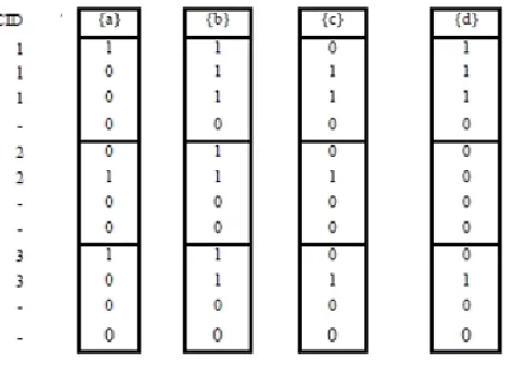
Step 1: Data Representation (Converting database to vertical bitmap): For efficient counting of support, SPAM algorithm uses a vertical bitmap representation of the data. A vertical bitmap is created for each item in the dataset, and each bitmap has a bit corresponding to each transaction in the dataset. The Database D in Table 5 is converted, into a vertical bitmap by setting (1) or (0) shown in Figure 1, where each candidate-1 item (such as a, b, c, d)) has a vertical column and each subsequence (e.g., CID1 = < {a, b, d}, {b, c, d}, {b, c, d}>) is mapped in the 1-event bitmaps. For example, the first transaction CID 1 the bitmap obtained after mapping to events a, b, c, d is: 1101, 0111, and 0111.

Figure 1: Vertical Bitmap of items in database

(19)

8

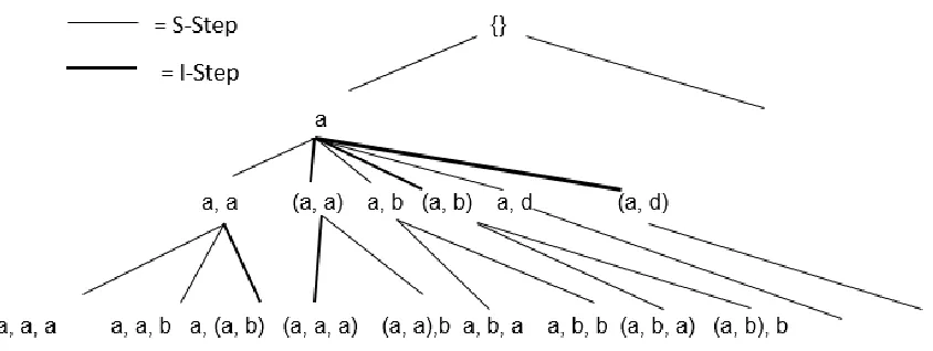
each suffix sequence to be extended with such as (a, b, and d) a sequence-extended children sequences generated in the S(sequence-extension)-Step of the algorithm (for example, from CID 1, aa, ab, ad are obtained respectively) and itemset-extended children sequences generated by the I(item-extension)-Step of the algorithm at each node (For example, from CID 1,(a, a),(a, b), (a, d) are obtained respectively). Thus, for the first subsequence of CID=1, the lexicographical tree for items a, b and d obtained is shown in the Figure 2, assuming a maximum sequence size of 3.

Figure 2: Lexicographic tree

(20)

9

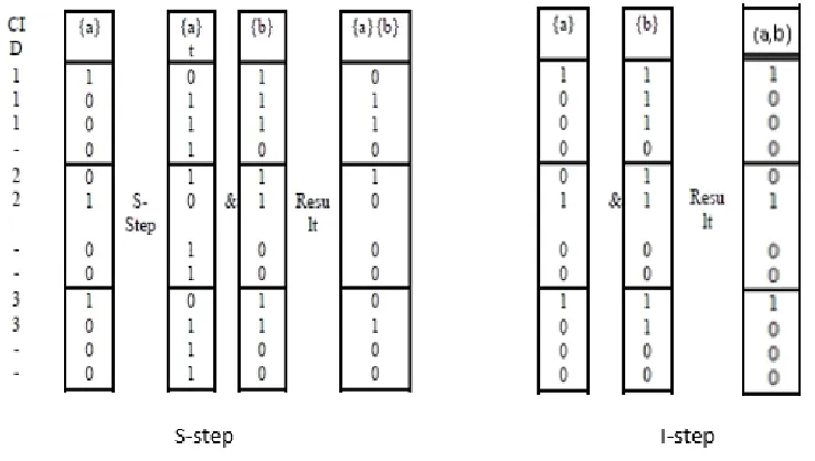
When the transformed bitmap ‘{a} s’ is obtained, the bit-AND operation is performed on ‘{a} s’ and {b} to get the result of S-step of ({a}, {b}). As support count of ({a}, {b}) was 4, the pattern ({a}, {b}) was considered as frequent.

Figure 3: The S-step and I-Step procedures

(21)

10

considered and suppose that S ({a}) = {a, b, c, d}, I ({a}) = {b, c, d}. The possible sequence-extended sequences are ({a}, {a}), ({a}, {b}), ({a}, {c}) and ({a}, {d}). Suppose that ({a}, {c}) and ({a}, {d}) are not frequent. By the Apriori principle, none of the following sequences can be frequent either: ({a}, {a}, {c}), ({a}, {b}, {c}), ({a}, {a, c}), ({a}, {b, c}), ({a}, {a}, {d}), ({a}, {b}, {d}), ({a}, {a, d}), or ({a}, {b, d}). Hence, when we are at node ({a}, {a}) or ({a}, {b}), so I-step or S-step is not performed for items c and d, i.e. S({a},{a}) = S({a},{b}) = {a, b}, I({a},{a}) = {b}, and I({a},{b}) = ∅. I-step Pruning prunes I-step children. For example, if the same node ({a}) described in the S-step pruning section. The possible itemset-extended sequences are ({a, b}), ({a, c}), and ({a, d}). If ({a, c}) is not frequent, then ({a, b, c}) must also not be frequent by the Apriori principle. Hence, I ({a, b}) = {d}, S ({a, b}) = {a, b}, and S ({a, d}) = {a, b}.

Advantage: It is the first algorithm to utilize a depth-first traversal for the search space in the tree which is combined with a vertical bitmap representation to store each sequence. Limitation: As SPAM uses a depth-first traversal of the search space, it is quite space-inefficient for smaller datasets.

1.3. WEB MINING

Web mining categorized into three different classes based on which part of the Web is mined. These three categories are (i) Web content mining, (ii) Web structure mining and (iii) Web usage mining (Vijayalakshmi et al., 2010)

(22)

11

(ii) Web structure mining: It is the process of discovering the structure of hyperlinks on the Web. Authoritative pages contain useful information and supported by several links pointing to it, which means that these pages are highly referenced. Web structure mining can exploit the graph structure of the web to improve the performance of the information retrieval and to improve classification of the documents.

(iii) Web usage mining: There are three types of log files that can be used for Web usage mining. Log files are stored on the server side, on the client side and the proxy servers. By having more than one place for storing the information of navigation patterns of the users makes the mining process more difficult. Some commonly used data mining algorithms for Web usage mining are association rule mining, sequence mining and clustering (Vijayalakshmi et al., 2010).

1.4. HIGH UTILITY ITEMSET MINING

The utility is introduced into pattern mining to mine for patterns of high utility by considering the quality (such as profit) and quantity (such as a number of items purchased) of itemsets. This has led to high utility pattern mining (Yao et al., 2004), which selects interesting patterns based on minimum utility rather than minimum support. High utility itemset refers to those set of items which has a high utility such as profit in a database. Web usage mining is to discover user traversal patterns of Web pages from Weblog records. For an example, a popular Website may register the Weblog records in the order of hundreds of megabytes every day from various users, which provide rich information about the Webpage importance. The utility is a measure of how “interesting” or “useful” a Web page is. As a result, it allows Web service providers to select user preferences of different traversal paths.

(23)

12

be the browsing time a user spent on a given page) and also the external(quality) utility value (which could be the end user’s preference).

Step 2: The utility of a web page is the product of internal and external utility in which a web page refers to an item, a traversal sequence refers to an itemset, the time a user spent on a given page X in a browsing sequence T is defined as utility denoted as u(X, T) (Zhou et al., 2007). The more time a user spent on a Web page, the more interesting it is to the user. Thus, utility-based web path traversal pattern mining is to find all the Web traversal sequences that have high utility beyond a minimum threshold.

Step 3: The challenge of utility mining is that it does not follow “downward closure property,” that is, a high utility itemset may consist of some low utility sub-itemsets. The two-phase algorithm proposed by (Yao et al., 2006) aimed at solving this difficulty which was described in the two phases. In Phase I, transaction-level utility is proposed and defined as sum of the utilities of all transactions containing X. High transaction-level utility sequences are identified in Phase I. A Transaction-level Downward Closure Property is that any subset of a high transaction-level weighted utility (TWU) itemset must also be high in transaction-level weighted utility.

Step 4: In Phase II, only one database scan is performed to filter out the high transaction-level weighted utility itemsets that are low utility itemsets. The size of candidate set is reduced by only considering the supersets of high TWU sequences.

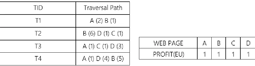
An example, the Utility based Web Traversal Pattern(UWTP) Mining Algorithm (Zhou et al., 2007), which extends the Two-Phase algorithm to traversal path mining problem. Input: A Traversal path database and a Profit table is given in Table 6, Candidate -1 Sequences C1= {A, B, C, D}; Minimum Utility Threshold = 12;

Output: High Utility Sequential Patterns

(24)

13

Table 6: A Traversal Path Database and Profit Table

From Step 2, The utilities of A was (2*1+1*1+1*1) = 4; B = (1*1+6*1+5*1) = 12; C = (1*1+1*1) = 2; D = (1*1+3*1+4*1) = 8; AB = (3+6) = 9; AC = 2; AD = 9; BC = 7; BD = 16; CD = 6; ABD = 10; ACD = 5; BCD =8; the transaction-level utility are T1 :3; T2:8; T3=5; T4=10.From the database in Table 6, From Step 3, the TWU sequences are A= 18; B= 21; C= 13; D= 23; AB= 13; AC= 13; BC= 8; BD= 18; CD= 13; ABD= 10; ACD= 5; BCD= 8. From Step 4, If the Minimum Utility Threshold = 12, then the High Utility Sequential Patterns generated are A, B, C, D, AB, AC, BD, and CD.

Advantage: The high utility traversal paths may assist Web service providers to design better web link structures, thus cater to the user's interests in the websites.

Limitation: Not confined to larger databases.

1.5. REAL LIFE SCENARIOS OF THE HIGH UTILITY MINING

Frequent itemsets may only contribute a small portion of the overall profit, whereas non-frequent itemsets may contribute a substantial portion of the profit. So, they are mined separately.

(25)

14

than the printer, but the value if the printer is high which can be profitable to the business owner. The utility is based on quality and quantity of an item in the database.

2. WEB LOG DATA: A sequence of web pages visited by a user can be defined as a transaction. Since the number of visits to a web page and the time spent on a webpage is different between different users, the total time spent on a page by a user can be viewed as internal utility and the webpage rating provided by the website can be measured as the external utility. The website designers and web service providers can catch the interests or behavior patterns of the customers by looking at the utilities of the page combinations and then consider re-organizing the link structure of their website to cater to the preference of users. Frequency is not sufficient to answer questions, such as whether a webpage is highly profitable, or whether a web traversal has a strong impact.

1.6. HIGH UTILITY SEQUENTIAL PATTERN MINING

(26)

15

profitable sequential patterns are retrieved, which are more informative for retailers in determining their marketing strategy. First, as with high utility itemset mining, the downward closure property does not hold in utility-based sequence mining. This means that most of the existing algorithms cannot be directly transferred, from frequent sequential pattern mining to high utility sequential pattern mining. Later with the advent of the sequence weighted utility, the Apriori property issue is resolved as the normal sequence utility does not hold the property but the weighted sequence utilities follows the Apriori property from which the high utility sequential patterns are generated. To effectively prune the search space, the concept of Sequence- Weighted Utility (SWU) (Liu et al., 2005) was proposed to serve as an over-estimate of the true utility of a sequence, which has the downward closure property. This SWU model is incorporated into the proposed framework, and a new model called Transaction based Sequence-Weighted Utility (TSWU) is introduced to effectively prune the search space. A sequence is regarded as a high utility sequence (HUS) if its SWU is no less than the minimum utility threshold. An SWU-based algorithm finds HUS’s and then identifies the high utility sequences from HUS and spends much time to filter out low utility sequences from HUSs, thus prolonging the execution time.

For example, USpan (Yin et al., 2012) is one of the high utility sequential pattern mining algorithms composed of lexicographic q-sequence tree, 2 concatenation mechanisms and 2 pruning strategies.

Input: A sequence database, Profit table, Minimum Utility threshold. Output: High Utility Sequential Patterns

Step 1: For utility-based sequences, the concept of the Lexicographic Sequence Tree is utilized to the characteristics of q-sequences, and come up with the Lexicographic Q Sequence Tree (LQS-Tree) to construct and organize utility based q-sequences.

(27)

16

I-Concatenation will occur. Otherwise, if the size increases by one, S-Concatenation is occurred. For example, <ea>’s I Concatenate and S-Concatenate with b result in <e(ab)> and <eab>, respectively. Assume two k-sequences ta and tb are concatenated from sequence t, then ta < tb if

i) ta is I-Concatenated from t, and tb is S-Concatenated from t, or

ii) both ta and tb are I-Concatenated or S-Concatenated from t, but the concatenated item in ta is alphabetically smaller than that of tb.

For example, <(ab)>, < ((ab)b)>, <(abc)> < (ab)b>, <(ab)c> < <(ab)d> .

Step 3: A lexicographic q-sequence tree (LQS-Tree) T is a tree structure satisfying the following rules: Rule1: Each node in T is a sequence along with the utility of sequence, while the root is empty and Rule 2: Any node’s child is either an I-Concatenated or S-Concatenated sequence node of the node itself. Rule 3: All the children of any node in T are listed in an incremental and alphabetical order.

Step 4: Additionally, if minimum utility threshold = 0, then the complete set of the identified high utility sequential patterns forms a complete LQS-Tree, with complete search space. USpan uses a depth-first search strategy to traverse tree to search for high utility patterns. Step 5: The I-Concatenation and the S-Concatenations are applied to the LQS Tree. Step 6: The depth and width pruning techniques are further applied to remove the unpromising candidates from the tree. An example explaining the USpan algorithm is mentioned in the section 2.4.2.

Advantage: It follows the bitmap representation like in SPAM algorithm which is suitable for larger datasets.

(28)

17

1.7. UNCERTAIN DATA

A common cause of uncertainty comes from measurement errors: the locations of users obtained through RFID (Radio Frequency Identification) (Sistla et al., 1998) or GPS (Global Positioning System) of moving objects are not precise (Khoussainova et al., 2006) data collected from sensors in habitat monitoring systems (such as temperature and humidity) and noisy (Deshpande et al., 2004). As an example, Table 7 shows the records of the ids of the speeding vehicles (Vehicle in the table) and the speed (Speed) captured by sensor nodes (SID) at a certain location (Loc.) and time (Time). Each record is given an occurrence probability (P) representing its confidence to be true. In this example, records R1 and R2 cannot appear in the same possible world; that is, R1 and R2 are exclusive as they occur on the same day and same time. R3 is independent with them; this means the generation rule containing R3 only is independent with generation rule {R1, R2}. There are six possible worlds for this uncertain database, as shown in Table 8, along with corresponding possible world’s occurrence probabilities.

RID SID TIME LOC VEHICLE SPEED PROB

R1 S1 2: 00PM L1 HB1235 120 0.7

R2 S2 2: 00PM L1 HB1238 150 0.2

R3 S3 3: 45PM L1 HB2568 170 0.9

Table 7: Speeding Vehicle Records

Possible World Occurrence Probability

W1 {φ} 0.01

W2 {R1} 0.07

W3 {R2} 0.02

W4 {R3} 0.09

W5 {R1, R3} 0.063

W6 {R2, R3} 0.18

(29)

18

It is assumed that the items occurring in a transaction are known for certain. However, this is not always the case. For instance, in many applications, the data is inherently noisy, such as data collected by sensors or in satellite images. In real-life applications, utility and probability are two different measures for an object (e.g., a useful pattern). The utility is a semantic measure which is based on the user’s prior knowledge and goals, while probability is an objective measure in which the object or pattern has existential probability. Up to now, most algorithms of High Utility Mining such as U-Mining (Yao et al., 2004), Two-Phase algorithm (Yao et al., 2006), HUI-Miner (Liu and Qu 2012), PHUI-UP (Lin et al., 2016) have been extensively developed to handle precise data, which are not suitable to mine the data with uncertainty. To the best of my knowledge, the proposed framework will be the first work to address the issue of Mining High Utility Itemsets from the uncertain web access sequence database.

Example 1: Measured values in sensor data applications are notoriously imprecise. An example is an ongoing project at Purdue University (Aggarwal et al., 2009) that tracks the movement of nurses to study their behavior. Nurses carry RFID tags (Chen et al., 2005) as they move around the hospital. Numerous readers located around the building report the presence of tags in their vicinity. The collected data is stored centrally in the form “Nurse2 in room6 at 10:10 am”. Each nurse carries multiple tags. Difficulties arise due to the variability in the detection range of readers; multiple readers detecting the same tag; or a single tag being repeatedly detected between two readers (e.g., between room6 and the hallway – is the nurse in room6 all the time, just that the hallway sensor is detecting his tag or is she actually moving in and out?). Thus, the application may not be able to choose a specific location for the nurse always with 100% certainty.

(30)

19

infeasible for a sensor database to contain the exact value of each sensor at any given point in time. Thus, the traditional model of a single value for a sensor reading is not a natural fit with this data (Agrawal 2009). Instead, a more appropriate model is one where the sensor attribute can be represented as a probability distribution reflecting the inherent uncertainties and interpolation between measurements. Overall, these kinds of emerging database applications require models which can handle uncertainty and semantics to define useful queries on such data. A major choice for each model is whether to

incorporate probability values at the tuple or attribute level. This leads to two slightly different approaches in modeling and representing uncertain data (Aggarwal and Philip 2009). There are two main approaches for modeling uncertain relational data. One approach (Tuple uncertainty) is to attach a probability value with each tuple – the probability captures the likelihood of the given tuple being present in the given relation (Aggarwal 2009). The probability values for different tuples are assumed to be independent of each other unless some dependency is explicitly given. These dependencies across tuples can be used to express mutually exclusive alternatives. Such tuples are called x-tuples. The Table 9 shows uncertainty information expressed using tuple uncertainty. The tuples for Carid = Car1 are grouped together in an x-tuple, so they are mutually exclusive. Thus, Car1 has problems with either Brakes or Transmission with probability 0.1 and 0.2 respectively.

Car Id Problem Probability

Car1 Car2

Brakes Tires

0.1 0.9 Car 1

Car 2

Transmission Suspension

0.2 0.8

(31)

20

The second approach (Attribute uncertainty) allows for probability values at the attribute level. Table 10 is expressed using Attribute Uncertainty. It should be noted that both models are similar, as they use possible world’s (existence of an item or not) semantics for probabilistic calculations and for verifying the correctness of operations.

Car Id Problem

Car1 {(Brakes,0.1), (Tires,0.9)}

Car2 {(Trans,0.2), (Suspension,0.9)}

Table 10: Example of a relation with Attribute Uncertainty

It is assumed that the items occurring in a transaction are known for certain data. However, it is not always the same case. For example, in many applications, the data seems to be uncertain particularly when it was from GPS or RFID, Sensors (Bernecker et al., 2009). Up to now most algorithms of High utility itemset mining are developed to read precise data, and are not useful for uncertain data. The proposed framework will be the first solution of retrieving the high utility sequential patterns from uncertain weblog sequences. The differences between certain and uncertain data were given in Table 11.

Certain Web access data Uncertain Web Access Data

The data is clean and can be used directly for the process of the mining

The data is inaccurate and needs to be preprocessed further for the mining.

Example:

Car Id Problem

Car1 {(Brakes), (Tires)}

Car2 {(Trans), (Suspension)}

Example:

Car Id Problem

Car1 {(Brakes,0.1), (Tires,0.9)}

Car2 {(Trans,0.2), (Suspension,0.9)}

(32)

21

Uncertainty in Sequential Pattern Mining:

In sequential pattern mining algorithms, one of the algorithms deals with the uncertain data was the U-PLWAP algorithm (Uncertain Pre-linked position coded web access pattern algorithm) (Kadri and Ezeife 2011). It is noted here that unlike in traditional, precise sequences where occurrence count of an item automatically contributes towards the support count of an item, the sum of the product of the existential probability values is used in arriving at support counts. An equally important observation with the uncertain data items is that items with the same label can have different existential probability values in single sequence (for example, < (a:0.1, b:0.3, c:0.4, a:0.5) > the a has multiple existential probability values in the same transaction). It is, therefore, important to record item’s label, occurrence count and the existential probability values to determine frequent sequences accurately. The steps of UPLWAP algorithm are (Kadri and Ezeife 2011): Step1: The U-PLWAP scans the sequence database to discover the frequent 1-sequences. This is done by adding up all existential probability values for each item whenever they occur in the database. Whenever an item is repeated in a sequence, it’s the higher existential probability is only added. The frequent 1-sequences are those items with counts greater than or equal to the minimum support threshold.

(33)

22

exists, otherwise, a right node is created and the count initialised to 1. If node already exists, its count is incremented by 1. The item label and its existential probabilities are read from the sequence database. Entries created in the header table are then used to link their corresponding nodes by traversing the U-PLWAP tree in a pre-ordered fashion (from root to left node first before right node).

Step4: The U-PLWAP tree created is then mined recursively using prefix conditional search until no more items found. The algorithm then backtracks to the null root to start mining for sequences starting with a fresh item from the header table. The example explaining for U-PLWAP algorithm is mentioned in the section 2.2.2.

Advantage: The PLWAP tree algorithm is implemented in the uncertain data with the same methodology.

Limitation: The algorithm does not apply on utility. The support count, which is the sum of the all existential probability values for each item, sometimes involve in low existential probabilities with high profitable value.

Uncertainty in High Utility Itemset Mining:

(34)

23

mine potential high utility itemsets (PHUIs) using a level-wise search. As it adopts a generate-and-test approach to mine PHUIs, it suffers multiple database scans. The “utility” can be viewed as the user-specified importance, i.e., weight, cost, risk, unit profit or value; but numerous discovered HUIs may not be the patterns required by a retailer to take efficient decisions, since traditional HUIM algorithms do not consider existence probabilities. Discovered patterns may be misleading if they have low existential probabilities. The PHUI-UP algorithm has two phases: In first phase, the HTWPUIs are found until no candidate is generated, and in the second phase, PHUIs are derived with an additional database scan.

Step 1:The proposed PHUI-UP algorithm takes input as Uncertain Transaction database and scans the database to find the TWU (Transaction Weighted Utilities) and the probabilities (PRO) values using the tuple based uncertainty model for all the 1-itemsets. The utility and transaction utility and the weighted transaction utilities are calculated. Step2: Once all 1-itemsets satisfies Transaction Weighted Utilities TWU of an itemset ≥ min utility threshold (MUT) and Probability (PRO) of an itemset ≥ min probability threshold (MPT), they are all put into the set of potential high transaction-weighted utilization itemsets (HTWPUIs). Then k is set to 2, and the candidates C2 are generated by applying Apriori-gen (HTWPUI1) using the lexicographic order of items.

(35)

24

PHUIs from the candidate HTWPUIs (completeness). An example is mentioned in the section 2.3.3.

Advantages: It is the first algorithm to mine high-utility itemsets from an uncertain transaction database.

(36)

25

1.8. THESIS PROBLEM AND CONTRIBUTIONS

(37)

26

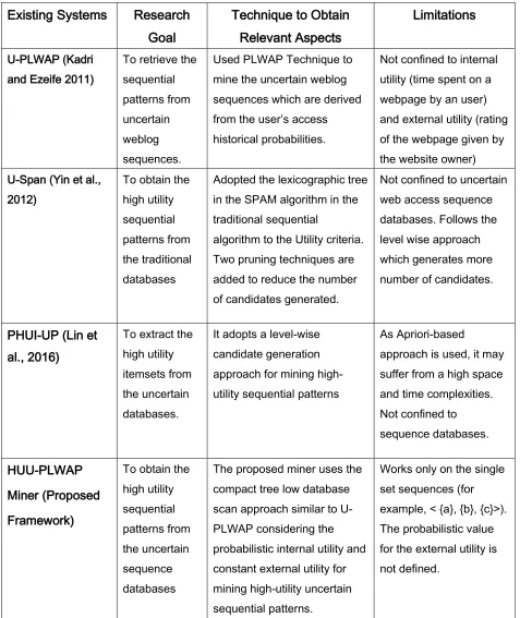
Existing Systems Research Goal

Technique to Obtain Relevant Aspects

Limitations

U-PLWAP (Kadri and Ezeife 2011)

To retrieve the sequential patterns from uncertain weblog sequences.

Used PLWAP Technique to mine the uncertain weblog sequences which are derived from the user’s access historical probabilities.

Not confined to internal utility (time spent on a webpage by an user) and external utility (rating of the webpage given by the website owner) U-Span (Yin et al.,

2012)

To obtain the high utility sequential patterns from the traditional databases

Adopted the lexicographic tree in the SPAM algorithm in the traditional sequential

algorithm to the Utility criteria. Two pruning techniques are added to reduce the number of candidates generated.

Not confined to uncertain web access sequence databases. Follows the level wise approach which generates more number of candidates.

PHUI-UP (Lin et al., 2016)

To extract the high utility itemsets from the uncertain databases.

It adopts a level-wise candidate generation approach for mining high-utility sequential patterns

As Apriori-based

approach is used, it may suffer from a high space and time complexities. Not confined to sequence databases.

HUU-PLWAP Miner (Proposed Framework)

To obtain the high utility sequential patterns from the uncertain sequence databases

The proposed miner uses the compact tree low database scan approach similar to U-PLWAP considering the probabilistic internal utility and constant external utility for mining high-utility uncertain sequential patterns.

Works only on the single set sequences (for example, < {a}, {b}, {c}>). The probabilistic value for the external utility is not defined.

(38)

27

The contributions of this thesis are therefore as follows: 1) Feature Contributions:

i. Developing a Sequential Pattern Miner for Uncertain Data with Internal and external Utility: HUU-PLWAP considers the items with lower existential probability whereas the U-PLWAP considers only find frequent sequential patterns. But there can be the pattern which is more profitable for the owner and least frequent, then these kind of patterns (which considers the internal (quantity) and external (quality) of the events in the sequence) are retrieved using the proposed miner

ii. Using Possible World Sequence of an Item model to derive internal utility for more profitable patterns: PHUI-UP (Lin et al., 2016) does not consider the internal probabilistic value where HUU-PLWAP calculates the uncertainty associated with the count of webpage retrieval along with the utility using on the sequence uncertainty model.

iii. More time and space efficient approach based on PLWAP compact tree structure that reudces multiple scan of the database: Existing approaches of High utility sequential mining such as USpan (Yin et al., 2012) have been extensively developed to handle precise data, which are not suitable to mine the sequence database with uncertainty and utility. Also, USpan (Yin et al., 2012) and PHUI-UP uses level wise approach for mining which can be more time to consume and a lot of memory consumption which can be improved by compact tree structure . iv. Probabilistic Internal Utility and Constant External Utility: The PHUI-UP considers

(39)

28

2). Procedural Contributions:

i. High utility sequential mining method for uncertainty sequence database: The proposed approach is the High utility sequential mining method for uncertainty sequence database. It follows the U-PLWAP methodology, but It considers both internal (time spent by the user on each web page which will vary in number) and external (the website rating given by the end users which is constant value) utilities of a web page which are not involved in U-PLWAP. It derives the internal utility value with uncertainty from the sequence uncertainty based model calculation. ii. Conditional Sequential Search: The HUU-PLWAP algorithm recursively mines the

HUU-PLWAP tree using the prefix conditional sequential search in the U-PLWAP along with uncertain internal utility and avoids the generation of the repetitive candidates, and multiple databases scans in the USpan. It also avoids the bitmap representation.

iii. HUU-PLWAP uses the compact tree low database scan approach: USpan is a vertical database bitmap transformation approach of the SPAM Algorithm (Ayres et al., 2002) in the sequential pattern approach in the frequent itemset mining and it uses the lexicographic tree approach for mining the patterns which can ne be more time consuming. The proposed miner applies the compact tree low database scan approach which is similar to the U-PLWAP tree (Kadri and Ezeife 2011) along with consideration of uncertain internal utility values and constant external utility values.

(40)

29

(represents the internal utility) to get the uncertain internal utilities values used for mining the high utility sequential patterns.

1.9. THESIS OUTLINE

(41)

30

2. RELATED WORK

Sequential pattern mining refers to the identification of frequent sub sequences in sequence databases as patterns. It provides an effective way to analyze the sequential data. The selection of interesting sequences is generally based on the frequency/support framework: sequences of high frequency are treated as significant. In the last two decades, researchers have proposed many techniques and algorithms such as APRIORI (Aggarwal and Srikanth 1995), FP-GROWTH ALGORITHM (Han et al., 2000), GSP (Srikant and Agrawal 1996), WAP (Pei et al., 2000), PL-WAP (Ezeife and Lu 2005) and so on, based on Apriori and Pattern growth methods for extracting the frequent sequential patterns, in which the downward closure property (also known as Apriori property) plays a fundamental role.

(42)

31

(section 2.1; section 2.2), High Utility Mining approaches (section 2.3) and High Utility Sequential Pattern Mining approaches (section 2.4) respectively.

2.1. SEQUENTIAL PATTERN ALGORITHMS IN CERTAIN DATA

Frequent Pattern Mining aims to discover how items purchased by customers in a supermarket with frequency no less than a user-specified threshold (m). For Example, Apriori algorithm (Aggarwal and Srikanth 1995) finds the set of frequent patterns iteratively by computing the support of each itemset in the candidate-1 itemset. An example is explained in Section 1.1. Another approach for Frequent Pattern Mining algorithm was Frequent Pattern tree (FP-Growth), which was explained in Section 2.1.1.

2.1.1. FP-GROWTH ALGORITHM (Han et al., 2000)

The problem of candidate set generation during frequent pattern mining process found that candidate set generation can be costly especially when many patterns are present and when such patterns are long.(Han et al., 2000) proposed a frequent mining algorithm, FP-growth, based on frequent pattern tree (FP-tree) data structure. The large database is compressed into FP-tree therefore removing repetitive database scan. This divide and conquer, conditional mining approach also remove candidate set generation.

Step 1: The FP-tree is built on the intuition that if frequent items are used to re-order items in the database, multiple transactions sharing same itemset can be represented by the same path in FP-tree by registering their counts.

Step 2: FP-tree is constructed after a first scan of the database is carried out where frequent items are found and ordered. The order is then used to enter items into the FP-tree during second scan.

(43)

32

Step 4: The conditional FP-tree is repeatedly mined when more than one frequent item is found.

Example: Input: The Transaction database in Table 13; minimum support is 3, Candidate 1-itemset = {a, b, c, d, e, f, g, h, i, j, k, l, m, n, o, p}.

Output: The Frequent Patterns.

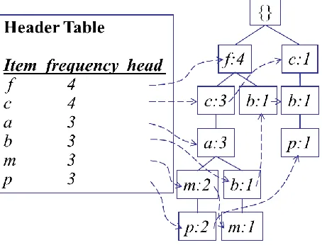
Step 1: The items are re-ordered according to descending order of frequent items (f:4, c:4, a:3, b:3, m:3, p:3). Items h, I, j, k, l has been removed from the database since they are not frequent.

TID ITEMS BOUGHT (ORDERED) FREQUENT ITEMS 100 f, a, c, d, g, i, m, p f, c, a, m, p

200 a, b, c, f, l, m, o f, c, a, b, m

300 b, f, h, j, o f, b

400 b, c, k, s, p c, b, p

500 a, f, c, e, l, p, m, n f, c, a, m, p

Table 13: Transaction database (Han et al., 2000)

The items are then inserted into the FP-tree in the ordered fashion as in Step 2 and the FP-tree generated is as given in Figure 4.

(44)

33

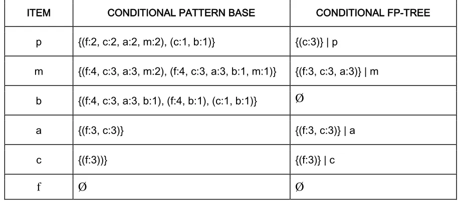
As per Step 3, Item p has 2 tree paths f:4, c:3, a:3, m:2, p:2 and c:1, b:1, p:1. Removing p and ensuring only counts for item p are present gives p’s conditional base tree: f:2, c:2, a:2, m:2, and c:1, b:1. Only item c make the minimum count of 3 (sum), therefore forms p’s conditional FP-tree (c: 3). Pattern ‘cp: 3’ is therefore frequent. The process is then repeated for all items on the header table. The conditional FP-tree is repeatedly mined as in Step 4 and the final output the frequent patterns generated are given in the Table 14.

ITEM CONDITIONAL PATTERN BASE CONDITIONAL FP-TREE

p {(f:2, c:2, a:2, m:2), (c:1, b:1)} {(c:3)} | p

m {(f:4, c:3, a:3, m:2), (f:4, c:3, a:3, b:1, m:1)} {(f:3, c:3, a:3)} | m

b {(f:4, c:3, a:3, b:1), (f:4, b:1), (c:1, b:1)} Ø

a {(f:3, c:3)} {(f:3, c:3)} | a

c {(f:3))} {(f:3)} | c

f Ø Ø

Table 14: The FP-growth mining process (Han et al., 2000)

Advantage: It resolved the problem of candidate set generation during frequent pattern mining process which was costly especially when many patterns are present and when such patterns are long.

Limitations: The execution time is more for the larger databases and it is not suitable for the non-sequential patterns.

2.1.2. GSP ALGORITHM (Srikanth and Aggarwal 1996)

(45)

34

the transactions are filtered by removing the non-frequent items. At the end of this step, each transaction consists of only the frequent elements it originally contained.

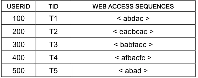
Step 1: This modified database becomes an input to the GSP algorithm. This process requires one pass over the whole database. It makes multiple database passes. In the first pass, all single items (1-sequences) are counted. From the frequent items, a set of candidate 2-sequences are formed, and another pass is made to identify their frequency. Step 2 The frequent 2-sequences are used to generate the candidate 3-sequences, and this process is repeated until no more frequent sequences are found. The two main parts of the algorithm are Candidate-Gen Joining phase, where the candidates for the next pass are generated by joining F (k-1) with itself from a given set of frequent (k-1)-frequent sequences F (k-1), and the Pruning phase which eliminates any sequence, at least one of whose subsequences is not frequent. Finally, non-frequent sequences are removed. Example: Input: Web Access Sequence Database in the Table15; minimum support is 3, Candidate 1-itemset = {a, b, c, d, e, f}.

Output: The Sequential Patterns.

USERID TID WEB ACCESS SEQUENCES

100 T1 < abdac >

200 T2 < eaebcac >

300 T3 < babfaec >

400 T4 < afbacfc >

500 T5 < abad >

Table 15: Web Access Sequence Database

(46)

35

{a, b, e}. The generate-and-test feature of candidate sequences in GSP has two phases explained in Step 2. During the join phase, candidate sequences are generated by joining Lk−1 with itself using GSP-join. From the seed set of three 1-sequences L1 = {a, b, e}, a candidate set C2 of twelve 2-sequences (3×3+ 3×2 2 = 12) is generated, giving an exploding number of candidate sequences, C2 = {aa, ab, ae, ba, bb, be, ea, eb, ee, (ab), (ae), (be) }, where parenthesis denote contiguous sequences (i.e., no time gaps), the algorithm then scans the sequence database for each candidate sequence to count its support, after the pruning phase, to get L2 = {ab:3, ae:4, ba:3, bb:3, be:4, (ab):3}, now GSP-join L2 with L2 (i.e., L2 GSP L2) to get C3 = {aba, abb, abe, bab, bae, b(ab), bba, bbe, bbb, (ab)a, (ab)b, (ab)e}, and so on, until Ck = {} or Lk−1 = {}. The set of mined frequent sequences is eventually fs = U kLk. To show an example of pruning the contiguous subsequence L3 = {(ab) c, (ab) d, a (cd), (ac) e, b (cd),bce}, then C4 = {(ab)(cd), (ab)ce}, and (ab)ce will be pruned because its contiguous subsequence ace is not in L3. The algorithm terminates when no new sequential pattern is found in a pass, or no candidate sequence can be generated.

Advantages: GSP employs a hash-tree to reduce the number of candidates that are checked for sequences. It is 2 to 20 times faster than Apriori-All.

Limitations: The GSP algorithm scans the original database and the problem of generating explosive candidate sets as in Apriori-like algorithms.

2.1.3. WAP TREE ALGORITHM (Pei et al., 2000)

(47)

36

2000).Instead of searching patterns level-wise as Apriori, WAP tree uses conditional search (a partition-based divide-and-conquer method), which narrows the search space by looking for patterns with the same suffix, and count frequent events in the set of prefixes with respect to condition as suffix. The main steps involved in this technique are summarized:

Step 1: The WAP-tree stores the web log data in a prefix tree format as the frequent pattern tree (FP-tree) for non-sequential data. The algorithm first scans the web log once to find all frequent individual events.

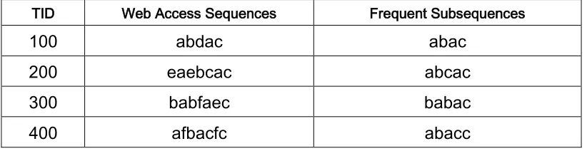
Step 2: Secondly, it scans the web log again to construct a WAP-tree over the set of frequent individual events of each transaction and finds the conditional suffix patterns. Step 3: Constructs the intermediate conditional WAP-tree using the pattern in Step 2. Step 4: Finally, it goes back to repeat Steps 3 and 4 until the constructed conditional. Example: Input: Web Access Sequence Database in the Table16; minimum support is 3, Candidate 1-itemset = {a, b, c, d, e, f}.

USERID WEB ACCESS SEQUENCES FREQUNET SUBSEQUENCES

100 abdac abac

200 eaebcac abcac

300 babfaec babac

400 afbacfc abacc

Table 16: A Sample database of web access sequences (Pei et al., 2000)

(48)

37

and a new child node c: 1 is created and inserted. The remaining sequence insertion process can be derived accordingly and shown in the Figure 5.

Figure 5: Example of web access pattern tree (Pei et al., 2000)

2.1.4. PL-WAP ALGORITHM (Ezeife and Lu 2005)

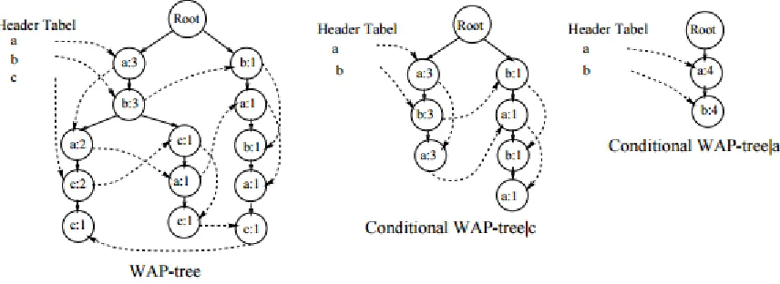
To eliminate the need of recursively construction intermediate trees in WAP tree, PLWAP algorithm was proposed, which uses position codes generated for each node such that antecedent/descendant relationships between nodes can be discovered from the position code (Ezeife and Lu 2005). The concept of binary tree is used in generating the position codes. The root has a position code of null. Starting from the root, all tree nodes are assigned a position code using the following rule. The position code of the leftmost child node is the position code of its parent concatenated with ‘1’ at the end; the position code of any other node is the same as appending ‘0’ to the position code of its closest left sibling (Ezeife and Lu 2005). The steps explaining the algorithm are:

(49)

38

Step 2: A second scan is then used to eliminate non-frequent events from the original sequences. These new sequences are then used to construct a PLWAP-tree with each node representing label, count and position code of the event along a particular path. Step 3: The PLWAP-tree is then traversed in a pre-ordered fashion starting from the root to the left sub-tree followed by the right sub-tree to build to build the header node linkages. Each event has a queue linking all its nodes in the order in which they are inserted. The head of each queue is registered in a header table for the PLWAP tree.

Step 4: The PLWAP algorithm then recursively mines the PLWAP tree using prefix conditional sequence search and generates the frequent sequential patterns.

Example: Input: Web Access Sequence Database in the Table17; minimum support is 75%, Candidate 1-itemset = {a, b, c, d, e, f}.

TID Web Access Sequences Frequent Subsequences

100 abdac abac

200 eaebcac abcac

300 babfaec babac

400 afbacfc abacc

Table 17: The Web Access Sequence Database (Ezeife and Lu 2005)

(50)

39

a: 3:1 and a: 1:101. The total count for ‘a’ is 4, making it a frequent 1-sequence. To find the next frequent sequence with ‘a’ as prefix, the PLWAP tree is rooted at b: 3:11 and b: 1:1011. The first occurrence of say ‘a’ in these sub-trees is then noted with the counts. For ‘a’ event, the following nodes are identified using b: 3:11 and b: 1:1011 as roots: a: 2:111, a: 1:11101 and a: 1:10111. Again ‘a’ occurs 4 times, making it frequent. Therefore, ‘aa’ is frequent sequence.

Figure 6: The PLWAP tree with the header linkages (Ezeife and Lu 2005)

The next 3-sequence with ‘aa’ as its prefix can be found by setting the root of the PLWAP tree to c: 2:1111, c: 1:111011 and c1:101111. There are no other events except ‘c’ with counts of c: 2:1111, c: 1:111011 and c1:101111, making it a total of 3, which makes ‘c’ frequent. Therefore, ‘aac’ is frequent. Shifting the root to c: 1:11111 gives no other frequent event. Step 4: The algorithm after recursive mining then backtracks to find other possible frequent sequence combinations at each level. The same procedure is followed and frequent sequences found are (a,aa, aac, ac, ab, aba, abac, abc, b, ba, bac, bc, c). Advantages: This algorithm includes efficiency in terms of I/O and memory utilisation since it eliminates the need to store intermediate WAP tree. The use of pre-order linking of header nodes of the same suffix tree also makes searching of nodes easier.

(51)

40

2.2. SEQUENTIAL PATTERN ALGORITHMS IN UNCERTAIN DATA

In the real-life applications, uncertainty may be introduced when data is collected from noisy data sources such as RFID, GPS, wireless sensors, and Wi-Fi systems (Aggarwal 2010) When applied to incomplete or in accurate data, traditional pattern mining algorithms (e.g., FIM, ARM) cannot be applied to discover the required information (Chun et al., 2007). Many algorithms have been developed to discover useful information in uncertain databases (De et al., 2013). The U-Apriori algorithm was first proposed to mine frequent itemsets in uncertain databases using a generate-and-test and breadth-first search approach (Chui et al., 2007). The Algorithm U-PLWAP tree (Kadri and Ezeife 2011) is constructed to mine the sequential patterns in the uncertain sequences without generating the candidate sequences, recursive construction of the intermediate tree and the necessity of the scan the sequence database repeatedly. All the mentioned algorithms are explained in the related work section 2.2.1 and 2.2.2.

2.2.1. U-APRIORI ALGORITHM (Chui et al., 2007)

(52)

41

Advantages: U-Apriori works like Apriori (downward closure property) and proves that it is also applicable in uncertain databases in which very subset of a frequent item set is frequent and vice versa.

Limitations: Generates enormous number of candidates and does not fit for large datasets.

2.2.2. U-PLWAP TREE ALGORITHM (Kadri and Ezeife 2011)

Uncertain Position Coded Pre-Order Linked Web Access Pattern (U-PLWAP) algorithm is proposed to provide solution in mining data that are associated with uncertainty. The uncertainty can be introduced, for example, in web logs, based on web log histories of different users. It is noted here that unlike in traditional precise sequences where occurrence count of an item automatically contributes towards the support count of an item, the sum of the product of the existential probability values are used in arriving at support counts. An equally important observation with uncertain data item is that items with the same label can have different existential probability values but higher value was considered. It is therefore important to record item’s label, occurrence count and existential probability values to accurately determine frequent sequences. The steps of algorithm are:

Step1: The U-PLWAP scans the sequence database to discover the frequent 1-sequences. This is done by adding up all existential probability values for each item whenever they occur in the database. Whenever an item is repeated in a particular sequence, higher existential probability is considered. The frequent 1-sequences are those items with counts greater than or equal to the minimum support threshold.

(53)

42

sequence. Each node contains the item’s label, multiple occurrence counts and their corresponding existential probability and position code, denoted as label: count: position code. Since similar labels with different existential probabilities in a path are merged into one node, each sequence read is identified by its sequence ID and recorded against the existential probabilities of its items in every node. A left node is created if no node already exists, otherwise, a right node is created and the count initialised to 1. If node already exists, its count is incremented by 1. The item label and its existential probabilities are read from the sequence database. Entries created in the header table are then used to link their corresponding nodes by traversing the U-PLWAP tree in a pre-ordered fashion (from root to left node first before right node).

(54)

43

updated sequence of cumulative products of existential probabilities. If no such item ’a’ is found, the algorithm backtracks to the last root and search for another item ‘b’. The process continues recursively until no more items are found. The algorithm then backtracks to the null root to start mining for sequences starting with a new item from header table.

Example: Input: Web Access Sequence Database in the Table18; minimum support is 25%, Candidate 1-itemset = {a, b, c, d, e, f}. Output: The Sequential Patterns.

From the Step1, Assuming the minimum support value is 1 out of 4 tuples that is 25% in Table 18. The expected support count values for all the items are calculated by adding up the existential probabilities of the item in each tuple. For example, the existential probability of item ‘a’ in user ID 10 is 1. The same value (1) is present in user IDs 20, 30 and 40. The expected support count of item ‘a’ is therefore given as 1 + 1 + 1 + 1 = 4. In the same vain, item ‘b’ has existential probabilities 0.5, 0.25, 0.5 and 1 in user IDs 10, 20, 30 and 40 respectively. The support count of item ‘b’ is therefore calculated as 0.5 + 0.25 + 0.5 + 1 = 2.25. The same process is used to find expected support counts for items ‘c’, ‘d’, ‘e’ and ‘f’ as: Item c = 0.75 + 0.25 + +0.75 + 0.5 = 2.25; Item d = 0.5 + 0.5 + 0.5 +0.25 = 1.75; Item e = 0.2 + 0.5 = 0.7 Item f = 0.2; Items ‘e’ and ‘f’ are non-frequent, so pruned.

User ID Web logs Frequent sub-sequences 10 (a:1, b:0.5, c:0.75, d:0.5) (a:1, b:0.5, c:0.75, d:0.5)

20 (a:1, b:0.25, d:0.5, c:0.25, d:0.5, e:0.2) (a:1, b:0.25, d:0.5, c:0.25, d:0.5) 30 (a:1, b:0.5, c:0.75, d:0.25, e:0.5) (a:1, b:0.5, c:0.75, d:0.25) 40 (b:1, c:0.5, a:1, d:0.5, c:0.5, f:0.2) (b:1, c:0.5, a:1, d:0.5, c:0.5)

Table 18 : Sample uncertain sequence (Kadri and Ezeife 2011)

(55)

44

a: 1, b: 0.5, c: 0.75, d: 0.5 is entered into the tree as the leftmost sub-tree since there no previously existing nodes. The count for each node initialised to 1 and their corresponding existential probability value are recorded. Each of the existential probabilities is also recorded against the sequence ID. The position codes for the nodes are given using the rule specified in step 2 of section 3.3 will explain the process. The second sequence a: 1, b: 0.25, d: 0.5, c: 0.5, d: 0.5 is read.

Figure 7: U-PLWAP Tree Constructed from the Example in the Table 18