ABSTRACT
AMAN, RONALD LEE. Evaluation and Modeling of Biodegradable Metallic Implants for Load-based Fixation. (Under the direction of Ola L. A. Harrysson and Denis R. Cormier.)
Biodegradable metal implant research is increasing in importance as a possible means to reduce complications associated with multiple surgeries in cases where load based fixation is necessary, but long term physical constraint of bone tissue is problematic. Recent advances in metallurgical studies of magnesium alloys have shown promise for their use as biodegradable implants, but the results of in vitro studies vary widely and do not compare well with in vivo studies.
In the second study, bone constructs consisting of simulated bone (polyacetal Delrin®), AZ31 alloy bone plates, and AZ31 bone screws were subjected to corrosion fatigue testing while immersed in Hanks Balanced Salt Solution for varying lengths of time. The test system imparted three different load mechanisms in 4 point bending orientation to 5 samples each over test durations of 0, 2, 4, 6, 8, 10, 14, 16, and 20 weeks. One set of samples was subjected to static loading, another set to dynamic or cyclic loading and the third set to no-load condition. After the corrosion process, corrosion products were removed via chromic acid etching and samples weighed and tested in a 4-point bend test. Bending strength, bending stiffness, and mass loss per week were recorded and compared for each sample.
Evaluation and Modeling of Biodegradable Metallic Implants for Load-based Fixation
by
Ronald Lee Aman
A dissertation submitted to the Graduate Faculty of North Carolina State University
in partial fulfillment of the requirements for Degree of
Doctor of Philosophy
Industrial Engineering Raleigh, North Carolina
2013 APPROVED BY:
_________________________________ Harvey A. West
_________________________________ Denis Marcellin-Little
_________________________________ C. Thomas Culbreth
_________________________________ Denis R. Cormier
Co-chair of Advisory Committee
_____________________________________ Ola L.A. Harrysson
ii
DEDICATION
iii
BIOGRAPHY
Ron is a two time graduate of North Carolina State University’s Edward P. Fitts Department of Industrial and Systems Engineering (B.S. 2002, M.S. 2004). His masters’ work focused on reverse engineering complex free-form surfaces and specifically aligning point cloud data from overlapping scan areas.
In 2004, Ron began Ph.D. studies and in 2005 took a full time Research Assistant position in the Furniture Manufacturing and Management Center at N.C. State University. During this time he participated in research related to furniture manufacturing, advanced manufacturing, additive manufacturing and was responsible for teaching undergraduate classes as well as managing manufacturing and computing laboratories. During this time Ron became interested in additive manufacturing and began research in two-phase electron beam melting, attempting to create metal matrix composites in a layer by layer process.
His research interest broadened to include biomedical applications of additive manufacturing. His dissertation work laid the groundwork for customized biomedical implants which can be custom tailored for each individual application.
iv
v
ACKNOWLEDGEMENTS
The work presented in this dissertation is the culmination of a long journey which would not have been possible without the help of a very large number of people. The support and friendship of the people listed below is the primary reason that this work was completed, and I cannot overstate their impact on my life:
To my co-advisors, mentors and friends Denis Cormier and Ola Harrysson, whose friendship and guidance I will always be thankful, and without their significant guidance and encouragement, this work would not have been completed. Ola’s dedication, drive, vast knowledge and interest in educating himself and those around him (even when seemingly they don’t want to be educated) is inspiring, and will lead to many very successful graduate students. His commitment to students’ success, academic integrity and progressing the state of the art are a model for all faculty to follow.
Denis’ exceptional research and academic vision inspires all that come into contact with him. He is always commenting or questioning things far in advance of what seemingly would make sense; I cannot count the number of ideas I have heard Denis comment about only to see them come to fruition 3-5 years later.
vi
all of his efforts in the future. Tom Culbreth’s willingness to help at all times and his absolute commitment to helping all students all of the time has been an incredible inspiration for me.
To Rusty King and Thom Hodgson, thank you for your inspiration, interest and helping to keep me on track. To the faculty of the Industrial and Systems Engineering department, thank you for all of the support and dedication.
To my fellow students that have had such an impact on my time here at N.C. State: Tim Horn, Molly Purser, Jessica Springer, Kyle Knowlson, Tushar Mahale, Harshad Srinivasan, Guhaprasanna Manogharan, Li Yang, and the many others that I have had the pleasure of knowing and interacting with, thank you for all you have done for me.
To Marcio Cerullo, thank you for all of your help in the nano lab. To Debbie Allgood-Staton, thank you for all of your support in making this happen.
To the Furniture Manufacturing and Management Center, this certainly would have not happened without all of the support and encouragement from those running and working in the center. To Steve Walker, thank you for all of the discussions we have had regarding the work here (and especially other things), and your encouragement to power through.
vii
viii
TABLE OF CONTENTS
LIST OF TABLES ... x
LIST OF FIGURES ... xi
1. INTRODUCTION ... 1
2. LITERATURE SURVEY ... 8
3. IN VITRO ANALYSIS OF STRENGTH AND CORROSION CHARACTERISTICS OF MAGNESIUM ALLOY (AZ31) IN HANKS SOLUTION ... 14
INTRODUCTION ... 14
METHODS AND MATERIALS ... 19
Methods ... 19
Materials ... 21
Sample Preparation ... 22
Test Rig Preparation ... 28
Sample Testing ... 33
RESULTS ... 36
DISCUSSION ... 42
RELATED AND FURTHER WORK ... 43
CONCLUSION ... 44
4. MECHANICAL PROPERTIES ANALYSIS OF AZ31 MAGNESIUM ALLOY UNDER DIFFERENT LOADING CONDITIONS IN HANKS BALANCED SALT SOLUTION ... 45
INTRODUCTION ... 45
MATERIALS AND METHODS ... 47
RESULTS ... 62
DISCUSSION ... 67
CONCLUSION ... 70
5. MODELING CORROSION OF AZ31 FOR OPTIMIZING CUSTOM OPEN REDUCTION INTERNAL FIXATION ... 72
INTRODUCTION ... 72
MATERIALS AND METHODS ... 75
MATHEMATICAL MODELING ... 77
RESULTS ... 84
DISCUSSION ... 86
FUTURE WORK ... 94
CONCLUSION ... 95
6. FUTURE WORK AND CONCLUSION ... 96
FUTURE WORK ... 96
ix
TABLE OF CONTENTS
Modeling ... 98 CONCLUSION ... 99
x
LIST OF TABLES
Table 3-1 Summary of the physical and mechanical properties of various implant materials in comparison to natural bone - reproduced
from (Staiger, Pietak et al. 2006) ...17
Table 3-2 Composition of AZ31 Alloy ...22
Table 3-3 Initial sample masses (grams) ...27
Table 3-4 Sample statistics, mass data in grams ...27
Table 3-5 Final sample masses, in grams ...40
Table 3-6 Sample mass gain in grams with average ...41
Table 4-1 Mass loss (grams) per week for cyclic loaded (CY), non-loaded (NL) and static loaded (ST) specimens ...63
Table 4-2 Time period comparisons of weekly average mass loss given in t statistic values (14 df) ...63
Table 4-3 Bending strength averages (Nm) for all samples, including those that broke during corrosion process ...64
Table 4-4 Bending strength averages (Nm) for all samples except those that broke during corrosion process ...65
Table 5-1 Bending Strength (Nm) comparison and corrosion depth (mm) estimate for cyclic loaded samples ...84
Table 5-2 Bending Strength (Nm) comparison and corrosion depth (mm) estimate for non-loaded samples ...85
Table 5-3 Bending Strength (Nm) comparison and corrosion depth (mm) estimate for statically loaded samples ...85
Table 5-4 Bending Strength (Nm) comparison and corrosion depth (mm) estimate for cyclically loaded samples with y =1.6 mm (assumed constant throughout test) ...88
Table 5-5 Bending Strength (Nm) comparison and corrosion depth (mm) estimate for non-loaded samples with y =1.6 mm (assumed constant throughout test) ...89
Table 5-6 Bending Strength (Nm) comparison and corrosion depth (mm) estimate for statically loaded samples with y = 1.6 mm (assumed constant throughout test) ...89
xi
LIST OF FIGURES
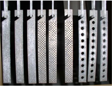
Figure 3-1 Sample configurations: Solid, large holes, and small holes ...23
Figure 3-2 Machining fixture in clamped position ...24
Figure 3-3 Machining fixture in open position showing aligning pins ...24
Figure 3-4 Dimensioned drawing of solid plate (top), large-hole plate (middle) and small-hole plate (bottom) (dimensions in mm) ...25
Figure 3-5 Test rig configuration showing samples hanging over empty test containers ...29
Figure 3-6 Environmental chamber used to maintain temperature conditions ...31
Figure 3-7 Test apparatus and samples immediately after start of test ...32
Figure 3-8 Test samples drying in environmental chamber following corrosion test and testing preparation ...34
Figure 3-9 ASTM F382-99 test set up with large span of 101.6 mm and small span of 25.4 mm ...35
Figure 3-10 ASTM F382-99 bending test during loading ...35
Figure 3-11 The average 0.2% offset proof load of samples versus time (Error bars are Standard Error) ...36
Figure 3-12 Average Bending Stiffness of samples versus time (Error bars are Standard Error) ...37
Figure 3-13 Average mass gain versus time, in grams, including linear trend line ...39
Figure 4-1 Simulated bone plate model ...48
Figure 4-2 Bone screw model based on a 3.5 mm cortical bone screw ...49
Figure 4-3 Simulated bone segments fabricated from Delrin ...49
Figure 4-4 Model of assembled bone construct ...50
Figure 4-5 Assembled bone construct...50
Figure 4-6 Model of test platform showing four test rows with containers for 15 samples ...52
Figure 4-7 Schematic of testing apparatus with construct in place ...53
Figure 4-8 Test rig immediately prior to initiation of loading. Note the aluminum cylinders (background top), Delrin loading rods with radius end showing, loading blocks, and constructs. HBSS with phenol red is easily seen, along with level-controlling overflow...54
xii
LIST OF FIGURES
Figure 4-10 Assembled and operating testing rig. Note: dynamic loading is in the foreground, static loading in the background and
no-load samples were in the middle ...56 Figure 4-11 Testing apparatus view from above showing individual testing
locations, orificed drains (center) and makeup water inlets at the sides. Note the corrosion on the samples to the right (after
2 weeks) as compared to the newly inserted 8-week samples ...58 Figure 4-12 ASTM F382-99 testing set up on universal test machine ...60 Figure 4-13 ASTM F382-99 4 point bend test at full displacement of a
non-corroded sample ...61 Figure 4-14 ASTM F382-99 4-point bend test showing permanent plastic
deformation of a non-corroded sample. Crosshead returned to
initiation location (Figure 4-11) ...62 Figure 4-15 Average Bending Strength vs. Exposure time in weeks.
Samples broken during corrosion process assumed to have
bending strength of 0 (Error bars are Standard Error) ...66 Figure 4-16 Average bending strength vs. exposure time in weeks.
Samples broken during corrosion process are not included ...67
Figure 5-1 Cross section of simple beam with dimensions b and h, and corrosion penetration x1, x2, x3, and x4 per side clockwise
around the cross section ...79 Figure 5-2 Graph of ∆I per mm of corrosion ...82 Figure 5-3 Estimate of the surface corrosion depth for different loading
conditions per exposure time ...86 Figure 5-4 Construct with lowest measured bending stiffness (14,571
N/m) and highest implied corrosion. Visual inspection shows much less corrosion penetration than predicted (predicted >
0.84 mm, original plate thickness = 3.2 mm) ...87 Figure 5-5 Micro CT image of construct 58 (cyclic loading) after 12 weeks
exposure to corroding medium. Measured pit depth is 2.11
mm, original thickness = 3.2 mm ...90 Figure 5-6 View of construct from various positions. Top left is a model
of the bone construct, top right is the approximate section plane of the radiographic slice in Figure 5-5, bottom is the
xiii
LIST OF FIGURES
Figure 5-7 Triangulated surface model of a boolean subtraction of a non-corroded sample and a non-corroded sample. Data reconstructed
1
1.
INTRODUCTION
Implants
The metallic medical implant market is growing approximately 9% per year and is currently estimated at about $27 billion (Yun, Dong et al. 2009). These implants are used for everything from bone fixation and reconstruction to stents used to open clogged arteries and microelectronics used for stimulation, control and data collection. Nearly all of these are made from stainless steels, cobalt chromium, or titanium alloys.
Biodegradable implants have recently been increasing in popularity. Recent advances in polymer science have created implantable polymer devices which can degrade over time and release elements which the body can either use internally or dispose of through the kidneys (Pietrzak, Eppley 2000, Suuronen, Pohjonen et al. 1998), and can effectively take the place of metallic implants (Lee, Oh et al. 2010). Examples of materials currently in use include poly(lactic acid) (PLLA, PDLLA), poly(glycolic acid) (PGA), poly(caprolactone) (PCL), poly(lactic glycolic acid) (PLGA), poly(methyl methacrylate) (PMMA) and more. These materials degrade in the body through hydrolysis and are eventually eliminated through respiration and urine, and can last anywhere from a few weeks to a few years (Middleton, Tipton 2000).
2
Biodegradable metallic alloys have been proposed using magnesium and magnesium alloys, and iron (Waksman, Pakala et al. 2008, Waksman, Pakala et al. 2007). These metals break down into corrosion products which the body can easily deal with and are, in most cases, required by the body for various biological processes. These metals have been proposed for use in bone fixation and reconstruction (bone plates) (Zhang, Xu et al. 2009), cement for implant stabilization (Yu, Wang et al. 2010), as stents (Waksman, Pakala et al. 2006), as base structures for tissue engineering (Witte, Ulrich et al. 2007, Gu, Zhou et al. 2010, Witte, Ulrich et al. 2007), and as biodegradable drug delivery vehicles (Di Mario, Griffiths et al. 2004).
Magnesium
3
among other components, were made from magnesium - and led to Volkswagen being the world’s largest consumer of magnesium in the 1960s and 1970s.
Magnesium is a common element found nearly everywhere on the earth, but not in its elemental state due to its high reactivity. Instead it is found as magnesium oxide (MgO) or magnesium chloride (MgCl2) and must be purified; normally using electrolysis of brine salts (Avedsian, Baker 1999). Approximately 68% of the magnesium produced in 1997 was used in alloying with either aluminum (~50%) or ferrous alloys (Avedsian, Baker 1999). Only approximately 30% was used in structural applications with die-casting being the major product (Avedsian, Baker 1999).
Pure magnesium has a density of 1.74 grams per cubic centimeter (g/cc) and compares to aluminum with a density of 2.70 g/cc and steels with densities greater than 7.7 g/cc. Magnesium has a melting point of 650 ºC, Young’s modulus of 45 GPa, and has a hexagonal crystal structure, meaning it is a relatively brittle metal. Magnesium is highly flammable and while easy to ignite in thin strips or powder is somewhat difficult to ignite in bulk. Once ignited, burning magnesium is very difficult to extinguish and typically requires suffocation using sand or earth.
Magnesium is the fourth most abundant mineral in the human body according to the National Institutes of Health (NIH). The NIH reports:
Magnesium is needed for more than 300 biochemical reactions in the body. It
helps maintain normal muscle and nerve function, keeps heart rhythm steady,
4
regulate blood sugar levels, promotes normal blood pressure, and is known to be
involved in energy metabolism and protein synthesis. There is an increased interest
in the role of magnesium in preventing and managing disorders such as
hypertension, cardiovascular disease, and diabetes. Dietary magnesium is absorbed
in the small intestines. Magnesium is excreted through the kidneys. (National
Institutes of Health 2009)
While dietary magnesium is essential to proper body function (Romani, Scarpa 2000, Rubin 2005, Rubin 2005), excess magnesium levels may be dangerous with symptoms including nausea, diarrhea, muscle weakness, extremely low blood pressure and irregular heartbeat. Magnesium is stored primarily in bones and is excreted through the kidneys when excess levels exist (National Institutes of Health 2009).
Alloying Agents
Magnesium alloys can be broadly broken down into three categories; pure magnesium with trace elements added, alloys containing aluminum (Zhang, Xu et al. 2009, Witte, Kaese et al. 2005, Witte, Fischer et al. 2006, Wen, Wu et al. 2009) and those free of aluminum. Alloying elements are generally added to improve the strength, fatigue resistance or corrosion resistance, or a combination of these properties. Magnesium alloys conform to the naming conventions outlined by ASTM using letter-figure combinations.
5
AZ31 are popular alloys often found in aerospace applications, and are available in cast, forged forms or as rolled sheets. The addition of aluminum improves strength and hardness and makes the alloy easier to cast. Zinc is added, especially in combination with aluminum, to improve strength at room temperature. With aluminum concentrations greater than 6% the alloy becomes heat treatable.
Alloys free of aluminum often contain rare-earth metals to improve strength at elevated temperatures. They also reduce weld cracking and improve porosity due to the elements’ effect on narrowing the freezing range of the alloy. Rare-earth elements normally are added in one of two forms, mischmetal or didymium. Mischmetal is a naturally occurring mixture of approximately 50% cerium and 50% lanthanum and neodymium, and didymium is a natural mixture of approximately 85% neodymium and 15% praseodymium.
Magnesium as an Implant
6
Magnesium and magnesium alloys generally corrode slowly in air (Song, Atrens 2004). However in environments which include chlorides in an electrolytic solution, such as the situation in the human body and saltwater, the corrosion rate is markedly higher. In fact, magnesium is often used as a sacrificial anode in these environments to protect other metals from corrosion. The corrosion rate in these environments can be controlled through several means: coatings applied to reduce fluid contact with the magnesium surface, impressed current, modification of the specific alloy or processing method, or control of the surrounding fluid pH.
Controlling the rate of corrosion is a major research issue with regard to biodegradable metal implants. High corrosion rates may cause premature loss of structural integrity of the implant, high evolution rate of hydrogen gas from the corrosion process, or overload the body with corrosion products. Structural integrity of the implant can be maintained by making the implant sufficiently large to allow for the degradation over the expected healing time. However the evolution of hydrogen is problematic because it is possible to exceed the absorption rate of the body, and may need to be removed by external means (i.e. needle extraction). The overall hydrogen adsorption rate in rats was 0.954 mL/hr (Piiper, Canfield et al. 1962), thus keeping hydrogen evolution less than this rate will minimize the likelihood of subcutaneous gas bubble formation. Optimizing the size, shape and alloy composition of potential implants is important to the success of biodegradable metallic implants and to the recipient’s physiological response to the implant.
7
8
2.
LITERATURE SURVEY
Magnesium was first proposed as a ligature in 1878 (Huse 1878). Polymer based ligatures did not yet exist, and the natural corrosion of magnesium in the body into magnesium hydroxide and the ability of the body to dispose of this made it an interesting candidate for use where fixation was required for limited periods of time. No subsequent operations to remove the ligature were required as the magnesium corroded away over a predictable amount of time.
In 1906 pure magnesium fixation plates were introduced by Lambotte (Witte et al. 2010). The plates were fixated using steel screws and resulted in rapid degradation, presumably through galvanic corrosion, within eight days. A small amount of work was done in the early part of the 20th century (McBride 1938), but interest soon faded in favor of stainless steel alloys which became available mid-century.
There has been renewed interest in magnesium as a biodegradable implant, and new alloys have been developed to reduce the high corrosion rate. Studies that compared different testing media (in vitro) (Xin et al. 2010) and alloys (Gu et al. 2009) showed widely variable results, and have not been consistent with in vivo results.
Biological Performance of Magnesium Alloys
9
predict in vivo corrosion results. In fact, the in vivo corrosion rate was about four orders of magnitude lower than in vitro results. In vitro testing consisted of placing several samples in a 25 liter solution of NaCl, MgSO4, MgCl2, CaCl2, in accordance with ASTM –D1141-98 for 24, 96, 192 and 240 hours at room temperature. In vivo corrosion rates were estimated by approximating the implant volume using voxelation of a 3D computer model reconstructed from 2D image layers captured using synchrotron-radiation-based microtomography (SRµCT). The 1.5 mm by 20 mm implants, cast then machined magnesium alloys, were in service for 18 weeks in the femora of guinea pigs. In vivo corrosion rates were estimated at 1.21x10⁻⁴ mm/year and 3.52x10⁻⁴ mm/year for LAE442 and AZ91D respectively. There are some questions regarding the controls used to determine the difference between in vivo and in vitro corrosion rates in this paper (Kannan, Raman 2008), including the use of simulated seawater used in the in vitro test and the temperature at which the in vitro test was carried out. It should be noted that it is well known that the corrosion rate increases with increased temperature in magnesium alloys, thus the in vitro corrosion rate in this study may very well be underestimated.
10
In 2008, Kannan and Raman (2008) evaluated a calcium containing magnesium alloy denoted AZ91Ca. Wu, Fan, Gao, Zhai, Zhu (2005) had previously reported that addition of calcium improved general corrosion performance and improved mechanical properties up to about 1 wt.%. The Kannan study showed that AZ91Ca (immersed in modified-Simulated Body Fluid (m-SBF)) corrosion performance and Ultimate Tensile Strength (UTS) was enhanced, when compared to a control group exposed to only air. The addition of calcium should not introduce new toxicity concerns as bone already contains large quantities of the element. Furthermore, it was suggested that the addition of calcium to the AZ91 alloy may accelerate calcium phosphate formation on the surface of the magnesium alloy, enhancing corrosion resistance and encouraging bone growth.
11
magnesium alloys containing rare earth elements in m-SBF is lower than in NaCl solutions, presumably caused by the addition of albumin in physiological concentrations.
12
favorable for biodegradation, and the grains tend to be dissolved more rapidly in the die cast sample leading to reduced mechanical properties.
Wang, Estrin and Zuberova evaluated the corrosion performance of AZ31 processed via Squeeze Casting (SC), Hot Rolling (HR) and equal channel angular pressing (ECAP) (Wang et al. 2008). They found that the SC samples, with grain sizes on the order of 450 µm, corroded more rapidly than the HR and ECAP samples with grain sizes of 15 µm and 2.5 µm respectively. The samples were suspended in Hanks solution, which was maintained at a pH of 7, for various lengths of time up to 20 days. The corrosion rate starts out relatively high and decreases over time for all three sample materials; SC starts at approximately 2 µm/day and decreases to less than 1 µm/day after 20 days. Similarly, the ECAP and HR sample degradation rates start at about 1.5 µm/day and 1.35 µm/day respectively after 1 day and decrease to approximately 0.8 µm/day after 20 days.
Zhang, et. al. (Zhang, Xu et al. 2009) reported an in vivo test that highlights the different degradation rates of magnesium alloys (Mg-Mn-Zn specifically) based on proximity to cortical and cancellous bone tissue. More degradation was noted in the marrow channel, presumably due to increased fluid access. Fibroblasts were noted at the bone/bone plate interface, but none were noted on the opposite side of the bone plate. No fibrous capsule or macrophage or giant cells were noted around the implant. Evaluation of the blood showed little change and no disorder to liver or kidneys was noted.
13
is greater than what the body can process. The zinc rich glasses showed a significantly denser and thinner corrosion surface after 72 hours in simulated body fluid, as compared to a porous and thicker surface for the lower zinc level samples. In addition, in animal studies, the zinc rich glasses showed no gas bubbles (implanted in soft tissue) as compared to magnesium samples which showed obvious gas bubble formation.
14
3.
IN VITRO
ANALYSIS OF STRENGTH AND CORROSION
CHARACTERISTICS OF MAGNESIUM ALLOY (AZ31) IN HANKS
SOLUTION
aRonald L. Aman, bOla L. A. Harrysson, cDenis Marcellin-Little, dDenis R. Cormier, eHarvey A. West, fC. Thomas Culbreth
a NC State University, [email protected]
b Associate Professor, Dept. of Industrial and System Engineering, NC State University. [email protected]
c Professor, Orthopedic Surgery, College of Veterinary Medicine, NC State
University. [email protected]
d Professor, Department of Industrial and Systems Engineering, Rochester Institute of Technology. [email protected]
e Research Assistant Professor, Dept. of Industrial and System Engineering, NC State University. [email protected]
f Professor, Dept. of Industrial and System Engineering, NC State University. [email protected]
Introduction
15
Magnesium and magnesium alloys have recently generated a significant amount of scientific interest for use in medical device implants and scaffold materials (Kirkland, Lespagnol et al. 2010, Yun, Dong et al. 2009, Staiger, Pietak et al. 2006, Witte, Eliezer et al. 2010, Gu, Zhou et al. 2010). Magnesium alloys have long been used in the aerospace and automobile industry due to their low weight (density of 1.74 g/cc) and moderate mechanical properties. However, these alloys typically have a high corrosion rate, especially in the presence of solutions containing chlorides, and are very susceptible to galvanic corrosion due to magnesium’s relatively anodic position in the electromotive series (Fontana, Green 1978). It is the property of high corrosion rate that generates much interest for this material in medical implants.
Interest in metallic bio-resorbable materials for implants has increased dramatically in recent years. Recent surveys of literature show substantial increases in the number of articles regarding bio-resorbable metal implants. Articles published by year range from 15 for all years up to and including 1990, to 23 published in 1999 alone, and 81 published in 2009 (ScienceDirect.com 2010). Of particular interest are magnesium and its alloys, which have an elastic modulus close to that of natural bone. This compares favorably relative to current implant materials (Staiger et al. 2006) for load based applications (see Table 3-1).
16
comprehensive review of biomaterials based on magnesium alloys is also available from Witte, et al. (2008).
Magnesium materials have shown good biocompatibility and resorbability in animal studies due to their corrosive breakdown into materials the body can process (Yun, Dong et al. 2009, Wang, Shinohara et al. 2009). Magnesium corrodes according to the following reaction:
Mg 2H O ↔ Mg OH H 3‐1
The above reaction is stepwise broken down into the following reactions:
Mgs ↔ Mg2 aq 2e‐ 3‐2
2H2O aq 2e‐ ↔ 2OH‐ aq H2 g 3‐3
Mg2 aq 2OH‐ aq ↔ Mg OH 2 s 3‐4
17
rate is less than that of the absorption by the body and would maintain structural integrity until the healing process is complete.
Table 3-1 Summary of the physical and mechanical properties of various implant materials in comparison to natural bone - reproduced from (Staiger, Pietak et al. 2006)
Properties Natural Bone Magnesium Ti Alloy Co-Cr alloy Stainless Steel
Density (g/cc) 1.8-2.1 1.74-2.0 4.4-4.5 8.3-9.2 7.9-8.1
Elastic Modulus
(GPa) 3-20 41-45 110-117 230 189-205
Compressive yield Strength (MPa)
130-180 65-100 758-1117 450-1000 170-310
Fracture Toughness (MPam1/2)
3-6 15-40 44-115 N/A 50-200
The corrosion rate of a wide variety of alloys has been studied in vitro (Wang, Estrin et al. 2008, Song 2007, Witte, Fischer et al. 2006, Zhou, Shen et al. 2010, Fekry, El-Sherif 2009, Wen, Wu et al. 2009). In vitro testing has been performed using many different testing methods and mediums (Xin, Hu et al. 2010), resulting in a wide range of estimates of corrosion rates. In addition, the actual corrosion rates observed during in vivo studies to date differ widely with in vitro models, up to 4 orders of magnitude (Witte, Fischer et al. 2006). A significant improvement would be realized if in vitro models and processes were developed that more precisely match in vivo results.
18
required. Various coatings have been employed including high purity magnesium (Salunke, Shanov et al. 2011), stearic acid (Ng, Wong et al. 2010), cerium-based coatings (Ng, Wong et al. 2010), dicalcium phosphate dihydrate (Hu, Wang et al. 2010), anodizing (Song 2007), TiO2 coatings (Wang, Wang et al. 2009), and various polymers including PCL (Wong, Yeung et al. 2010). The distinct disadvantage of a coating process used to protect the magnesium alloy in this case is that a failure at any point in the coating could result in premature and unpredictable failure of the implant.
Alloying elements with magnesium have long been studied for use in the transportation sector. The use of commercially available magnesium alloys, such as AZ31 with 3 wt% aluminum and 1 wt% zinc, and AZ91, with 9 wt% aluminum and 1 wt% zinc has been considered for implants. The distinct advantage of AZ91 as compared with AZ31 is the reduced rate of hydrogen evolution and implied reduction of corrosion rate. While the hydrogen evolution rate is considered similar to what the human body can tolerate without large gas bubbles forming (Song 2007), the long term effects of the higher concentration of aluminum have not been fully evaluated. Rare earth elements have been added to further reduce the corrosion rate of magnesium alloys with some success (Witte, Fischer et al. 2006), but long term toxicity studies have not yet been performed for these alloys.
19
studies have surfaced which evaluate magnesium alloy corrosion with different processing histories (Wang, Estrin et al. 2008), and the influence of microstructure (Kannan 2010).
To our knowledge, there is no literature which studies the effect of corrosion on the strength of AZ31 magnesium alloy in Hank’s solution over the expected life of a load bearing implant. The objective of this research is to quantify the change in mechanical properties of magnesium alloy (AZ31) plates over time submerged in a Hanks Balanced Salt Solution.
Methods
and
Materials
The materials used to perform the test were purchased off the shelf from a commercial supplier. The testing performed was derived from an ASTM standard test F382-99, Standard Specification and Test Method for Metallic Bone Plates. The objective of the testing was to
quantify the load capabilities of AZ31 alloy subjected to various immersion durations in a corrosive environment.
Methods
ASTM F382-99 provides terminology and definitions to support bone plate testing which are listed here for completeness:
0.2% Offset Displacement, q (in) – permanent deformation equal to 0.2% of the center loading span distance.
Bending Strength (Lb-in) – the bending moment necessary to produce a 0.2%
20
Bending Structural Stiffness, EIe (Lb-in2) – the bone plate’s normalized effective bending stiffness that takes into consideration the effects of the test set-up configuration.
Bending Stiffness, K (Lb/in) – the maximum slope of the linear elastic portion of the load versus load-point curve when tested.
Bone Plate Width, w (in) - the width of the bone plate.
Center Span, a (in) – distance between the two loading rollers.
Fracture Load, Fmax (Lbs) – the applied load at the time when the bone plate
fractures.
Loading Span, h (in) – distance between the loading roller and the nearest
support.
Proof Load, P (Lbs) – the applied load at the intersection point of 0.2% offset curve from the Bending Stiffness curve and the observed data.
The Bending Structural Stiffness is determined by the following expression:
2 3
12 3‐5
21
2 3‐6
The proof load was found by finding the intersection of the 0.2% offset curve and the load versus displacement data obtained from the test. The 0.2% offset curve was found by performing a linear regression on the most linear region of the test data and shifting 0.2% in the abscissa. The linear regression was performed in MATLAB® R2009a using a proprietary regression algorithm and choosing an arbitrary minimum number of points of 1000, representing approximately 17.8 newtons and approximately one mm of displacement. To automate the data analysis, a program was written in MATLAB® which found the best fit regression with the steepest slope. The linear regression was performed iteratively in ten point increments along the data in order to find the steepest slope region.
To find the proof load, the 0.2% offset curve intersection with the load-displacement data was found. This was performed using MATLAB® and automated to avoid personal judgment errors.
Materials
22
AZ31B-O alloy was procured from Magnesium Elektron N.A. (Madison, Illinois) in sheet sizes of 0.3 meters by 1.22 meters by 3.2 mm thick. The chemical composition was certified to be in accordance with AMS-4375K and QQ-M-44B as per Table 3-2.
Table 3-2 Composition of AZ31 Alloy
Al Zn Mn Ca Cu Fe Ni Si Others
(each) Others (Total) Magnesium
Min 2.5 0.7 .2 - - - -
Max 3.5 1.3 1.0 0.04 0.05 0.005 0.005 0.05 0.1 0.3 Balance
SamplePreparation
Because corrosion is proportional to the surface area exposed to the testing medium, three sample types were prepared: one solid, one with large holes simulating a bone plate, and one with a large number of holes to simulate a mesh structure. The surface areas of the three sample types were calculated using the SolidWorks Computer Aided Design (CAD) software.
Samples for the corrosion test were prepared by cutting the 0.3 meter by 1.22 meter sheets into 160 mm by 19.1 mm (length by width) sizes using a powered sheet metal shear. The shear was fit with a jig to ensure similar sample sizes and all samples were cut at one time.
23
edge was above the vise face. A 25.4 mm diameter insert cutter was then used to cut the edge of the samples to remove the sheared edge. This resulted in one cleanly machined longitudinal edge.
The samples were further machined by placing them in a fixture with the previously machined edge against a pair of reference pins and held in place via clamping pressure of three screws. The bottom piece of the fixture was made from aluminum stock drilled with holes to receive two 6.3 mm pins for alignment and three holes to receive screws to hold in place the top clamping part of the fixture. The top portion of the fixture was made from steel bar stock with the underside machined with a groove to ensure even clamping force on the magnesium samples and prevent samples from moving during the machining process.
24
Samples, two at a time, were loaded into the machining fixture, fitted tightly up against the locating pins in the center, and allowed to protrude past the ends of the clamping fixture (Figure 3-2 and Figure 3-3). A CNC program was written to machine the profile of the samples around the three un-machined edges (thus finishing all four edges, including the first edge that was machined previously) using a 6.3 mm flat end mill. This process ensured a consistent surface finish at the edges of the samples and a consistent size of 15.9 mm wide by 149.2 mm long. The profile of the sample included a slot at the top of the sample to aide in hanging during the testing. The edges were machined square except for the inlet and outlet surfaces of the hook which were given a radius of 1.5 mm to ease assembly of the test rig.
Figure 3-2 Machining fixture in clamped position
25
For samples with holes, a hole-drilling routine was added to the program. Large-holed samples were drilled with a 6.3 mm drill bit on the central axis of the sample a total of 10 times, evenly spaced across the face. The small-holed samples were drilled with a 1.88 mm drill bit in a repeat pattern resulting in 156 small holes evenly distributed across the face.
26
Burrs caused by the machining process were removed using a handheld de-burring tool to avoid injury during assembly of the test rig. The samples were also blown off with compressed air to remove the machining coolant, and stacked on paper towels to further remove moisture introduced during the machining process.
During the machining process, a machining coolant was used to reduce heat build-up on the tool and samples, to flush chips away from the surfaces being machined, and to minimize any fire hazard due to the small magnesium chips and the heat generated from cutting them. The cutting fluid was a water-based coolant and thus caused a dark gray oxide layer to form on the faces of the samples. This was machined away using an abrasive process with 150 grit paper. The surfaces of all of the samples were sanded in a consistent manner until all traces of oxide layer were removed and virgin metal was visible.
27
Table 3-3 Initial sample masses (grams)
Week
Solid (g) Small hole (g) Large Hole (g)
Sample # Sample # Sample #
1 2 3 1 2 3 1 2 3
0 12.678 12.764 12.771 9.942 9.870 9.950 10.979 10.931 10.940
2 12.770 12.765 12.753 9.834 9.868 10.007 10.950 10.910 10.923
4 12.716 12.744 12.763 9.889 9.910 9.951 10.959 11.001 10.948
6 12.715 12.698 12.810 9.928 9.880 9.885 10.991 10.964 10.932
8 12.757 12.712 12.718 9.849 9.978 9.894 10.899 10.940 10.933
10 12.739 12.712 12.744 9.969 9.968 9.999 10.937 10.975 10.945
12 12.724 12.689 12.720 9.816 9.936 9.919 10.954 10.928 10.904
14 12.814 12.769 12.793 9.913 9.898 9.977 10.914 10.880 10.920
16 12.721 12.783 12.678 9.994 9.892 9.988 10.929 10.954 10.935
18 12.696 12.748 12.787 9.895 9.962 10.015 10.850 10.950 10.953
20 12.806 12.723 12.799 9.939 9.904 9.958 10.880 10.919 10.957
Table 3-4 Sample statistics, mass data in grams
Solid Small Hole Large Hole
Theoretical
Mass (g) 12.784 9.998 10.980
Mean
Mass (g) 12.746 9.927 10.934
SD 0.038 0.053 0.032
Max 12.814 10.015 11.001
Min 12.678 9.816 10.850
28
TestRigPreparation
The test rig consisted of a tower constructed of extruded aluminum sections. The vertical section held a motorized linear slide to allow vertical translation of the samples during the test. The test rig was assembled using off-the-shelf materials, including a 24 volt DC gear motor and several custom-made connectors from the motor to the test platform.
The samples were moved vertically in their individual tanks of Hanks Solution at a frequency of 2 cycles per minute. Each cycle resulted in the sample being moved up 6.3 mm from the bottom position and then back down to the bottom position.
29
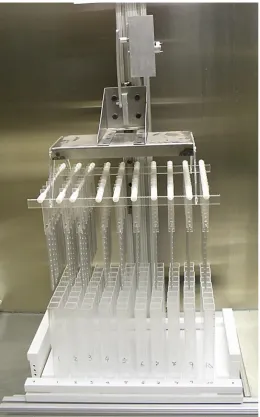
Figure 3-5 Test rig configuration showing samples hanging over empty test containers
30
samples. Ten rods were placed on the hanging system to allow for a total of 90 sample locations (ten rods with nine sample locations on each rod). Each rod contained three solid samples, three large-hole samples, and three small-hole samples. This represented the number of samples to be tested at each testing interval.
Testing containers were devised and constructed using an acrylic sheet and extruded acrylic square tubing. The square tubing was cut into lengths of 203 mm, and the parts were de-burred and cleaned in preparation for assembly. A base of 6.3 mm thick acrylic sheet was cut to 38.1 mm width and 279.4 mm length. Each row of nine cut extruded tubes was then attached to the acrylic sheet using adhesive, creating a series of containers capable of holding approximately 100 mL of fluid each. The containers measured approximately 25.4 mm by 25.4 mm (outside) by 203 mm high. The nine individual containers represent the number of samples to be tested at each testing interval.
31
Figure 3-6 Environmental chamber used to maintain temperature conditions
32
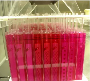
Figure 3-7 Test apparatus and samples immediately after start of test
33
during the Friday to Monday interval. The Monday to Tuesday interval showed the least evaporation.
At testing intervals of two weeks, the Hanks solution was removed from each test container, and the test container was rinsed with water. Each container was then refilled with fresh Hanks Solution. One set of nine test specimens was removed for testing, and the remaining samples were again submerged in the test solution.
SampleTesting
34
Figure 3-8 Test samples drying in environmental chamber following corrosion test and testing preparation
35
reversed and the unload rate was increased to 5.08 mm per minute. The load versus displacement data were recorded for each sample and retained for evaluation.
Figure 3-9 ASTM F382-99 test set up with large span of 101.6 mm and small span of 25.4 mm
36
Results
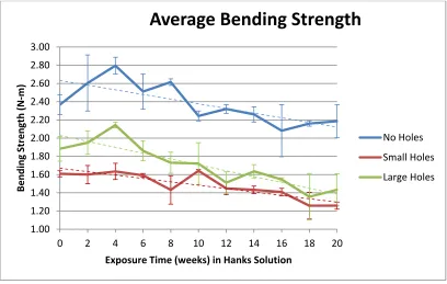
The bending strength (Figure 3-11) showed generally decreasing trends over time as expected due to corrosion. Bending strength for samples with no holes decreased from an average of 2.37 N-m to approximately 2.19 N-m over the 20 week test, however this was not statistically significant (t(4) = 1.48, p > 0.05). The no-hole samples retained approximately 92% of their original bending strength. The large-hole sample average bending strength decreased from 1.88 N-m to 1.43 Nm, retaining approximately 76% of the original bending strength (t(4) = 3.50, p < 0.05 (two-tailed)). Small-hole samples average bending strength decreased from 1.61 N-m to 1.26 N-m over the same 20 week test, retaining approximately 78% of the original bending strength (t(4) = 11.73, p < 0.05 (two-tailed).
Figure 3-11 The average 0.2% offset proof load of samples versus time (Error bars are Standard Error)
1.00 1.20 1.40 1.60 1.80 2.00 2.20 2.40 2.60 2.80 3.00
0 2 4 6 8 10 12 14 16 18 20
Bending Strength (N ‐ m)
Exposure Time (weeks) in Hanks Solution
Average
Bending
Strength
No Holes
Small Holes
37
The average bending stiffness (Figure 3-12) for no-hole samples decreased from 90,800 N/m to 78,057 N/m, retaining approximately 86% of the stiffness over the measurement period (t(4) = 5.19, p < 0.05 (two-tailed)). Large-hole sample stiffness decreased from 65,376 N/m to 48,830 N/m, retaining approximately 75% of the stiffness (t(4) = 3.39, p < 0.05 (two-tailed)), and small-hole sample stiffness decreased from 42,086 N/m to 30,232 N/m, retaining approximately 72% of the original stiffness (t(4) = 11.16, p < 0.05 (two-tailed)).
Figure 3-12 Average Bending Stiffness of samples versus time (Error bars are Standard Error)
20.00 30.00 40.00 50.00 60.00 70.00 80.00 90.00
0 2 4 6 8 10 12 14 16 18 20
Average
Bending
Stiffness
(kN/m)
Exposure Time (weeks) in Hank's Solution
Average
Bending
Stiffness
No Holes
Small Holes
38
The mass of the samples (Figure 3-13) as measured after immersion, rinsing and drying overnight showed generally increasing trends over time. The mass increased due to the accumulation of corrosion products on the surface of the samples. The decrease in proof load and average bending stiffness as well as the increase in mass are as expected.
39
Figure 3-13 Average mass gain versus time, in grams, including linear trend line
0.000 0.100 0.200 0.300 0.400 0.500 0.600 0.700
2 4 6 8 10 12 14 16 18 20
Average
mass
gain
per
sample
(grams)
Weeks exposed to Hanks Solution
Solid
Small Holes
40
Table 3-5 Final sample masses, in grams
Week
Solid (g) Small hole (g) Large Hole (g)
Sample # Sample # Sample #
1 2 3 1 2 3 1 2 3
0 12.678 12.764 12.771 9.942 9.870 9.950 10.979 10.931 10.940
2 12.827 12.817 12.822 9.854 9.899 10.034 11.022 10.942 10.969
4 12.864 12.793 12.814 9.890 9.941 10.014 10.962 11.077 10.948
6 12.811 12.852 13.145 9.978 9.928 9.881 11.144 11.026 10.946
8 12.782 12.788 12.701 9.933 10.025 10.343 10.914 11.357 11.011
10 12.770 13.109 13.007 10.155 10.174 10.170 11.073 11.158 11.509
12 12.864 12.770 13.031 10.405 10.088 10.088 11.313 11.242 11.390
14 13.041 13.262 13.348 10.000 9.996 10.296 11.449 10.862 11.128
16 12.757 12.929 13.323 10.254 10.165 10.179 11.128 11.156 11.168
18 13.150 13.149 13.096 10.691 10.415 10.334 10.835 11.444 11.953
41
Table 3-6 Sample mass gain in grams with average
Week
Solid (g)
Avg
(g)
Small hole (g)
Avg
(g)
Large Hole (g)
Avg
(g)
Sample # Sample # Sample #
1 2 3 1 2 3 1 2 3
0 0.000 0.000 0.000 0.000 0.000 0.000 0.000 0.000 0.000 0.000 0.000 0.000
2 0.057 0.052 0.069 0.059 0.020 0.031 0.027 0.026 0.072 0.032 0.046 0.050
4 0.148 0.049 0.051 0.083 0.001 0.031 0.063 0.032 0.003 0.076 0.000 0.026
6 0.096 0.154 0.335 0.195 0.050 0.048 ‐0.004 0.031 0.153 0.062 0.014 0.076
8 0.025 0.076 ‐0.017 0.028 0.084 0.047 0.449 0.193 0.015 0.417 0.078 0.170
10 0.031 0.397 0.263 0.230 0.186 0.206 0.171 0.188 0.136 0.183 0.564 0.294
12 0.140 0.081 0.311 0.177 0.589 0.152 0.169 0.303 0.359 0.314 0.486 0.386
14 0.227 0.493 0.555 0.425 0.087 0.098 0.319 0.168 0.535 ‐0.018 0.208 0.242
16 0.036 0.146 0.645 0.276 0.260 0.273 0.191 0.241 0.199 0.202 0.233 0.211
18 0.454 0.401 0.309 0.388 0.796 0.453 0.319 0.523 ‐0.015 0.494 1.000 0.493
42
Discussion
The nine samples collected in week four showed generally uniform corrosion with some evidence of pitting corrosion. Samples collected in week six showed generally uniform corrosion over the entire exposed surface. Pitting corrosion was evident in week six, but had not become a major source of corrosion products on the surface. In week eight, large scale corrosion products had accumulated on two of the nine samples - one with large holes and one with small holes. The corrosion accumulation was approximately 10 mm in diameter and 6 mm in thickness. The surrounding areas of the magnesium were heavily corroded and showed considerable pitting corrosion.
Samples evaluated after week eight generally showed results similar to those of week eight. Of note, several test specimens exhibited very little corrosion, even after 18 or 20 weeks in HBSS. This can be attributed to several factors, including the inherent variability in the corrosion process, the corrosion mechanism (primarily pitting corrosion) which is driven by metal association with chloride ions, and the micro-galvanic corrosion process which is dependent on differential of galvanic activity between the grain boundaries and the grains themselves.
43
products broke down, the load would then continue to increase. To eliminate these artificial affects, corrosion products at the points of support fixture and loading fixture interfaces with the test specimen were removed after week six testing. The corrosion products were removed using a mechanical scraping action with a steel blade.
Overall a gradual reduction in bending stiffness and bending strength can be attributed to increasing corrosion penetration over time. Considering the consolidation time for long bone fractures in children is 5 to 25 weeks (Berger, De Graaf et al. 2005) with a mean of 12 weeks, the bending strength retention between 76% and 92% measured in this study suggests AZ31 magnesium alloy could be a good candidate as a resorbable fixation material for orthopedic applications.
Related
and
Further
Work
44
in the first week of testing, when there was not an observable corrosion layer to obscure visual observation.
While the AZ31 alloy shows relatively slow degradation in strength over time in Hanks Balanced Salt Solution in this test, applications for load bearing fixation would be subject to variable loading over the course of healing. Future work should consider loading effects on strength retention and corrosion rate. Other corrosion mechanisms (other than galvanic, micro galvanic and general corrosion) may affect the corrosion rate and strength retention, and should be considered. Other corrosion mechanisms worthy of consideration include Stress Corrosion Cracking (SCC) and fatigue corrosion just to mention two.
Conclusion
45
4.
MECHANICAL PROPERTIES ANALYSIS OF AZ31 MAGNESIUM
ALLOY UNDER DIFFERENT LOADING CONDITIONS IN HANKS
BALANCED SALT SOLUTION
aRonald L. Aman, bOla L. A. Harrysson, cDenis Marcellin-Little, dDenis R. Cormier, eHarvey A. West, fC. Thomas Culbreth
a NC State University, [email protected]
b Associate Professor, Dept. of Industrial and System Engineering, NC State University. [email protected]
c Professor, Orthopedic Surgery, College of Veterinary Medicine, NC
State University. [email protected]
d Professor, Department of Industrial and Systems Engineering, Rochester Institute of Technology. [email protected]
e Research Assistant Professor, Dept. of Industrial and System Engineering, NC State University. [email protected]
f Professor, Dept. of Industrial and System Engineering, NC State University. [email protected]
Introduction
The service life of an implant is important to consider when designing a custom implant for reconstruction and fixation. Load bearing biodegradable metallic implants have special considerations in this light, since they are designed to degrade over time, and thus the functionality is intentionally reduced by corrosion. Understanding corrosion rates in the various conditions which the implant is expected to perform is important to reduce risk of premature failure in place, and to avoid excess exposure to degrading implant materials.
46
estimate corrosion current density. These test methods can provide estimates of corrosion rate in a short period of time by accurately measuring potential and electron flow. While the data can be collected easily, interpretation is complex.
Simple immersion tests evaluate the corrosion rate by leaving the test specimen in a container with testing medium for some time. These tests take longer and require maintenance of test conditions over long periods of time; however, the corrosion rates can be more meaningfully interpreted.
Corrosion rate plays an important role in determining the expected life of a bio-degradable implant, however other factors such as fatigue life and static stresses may play a large role as well (Song, Atrens 2004). Corrosion fatigue life is likely to be shorter than both corrosion life and the fatigue life due to interaction of both corrosion and fatigue (Nan, Ishihara et al. 2008, Kang, Yao et al. 2009), yet little information is available about this phenomenon with magnesium alloys.
47
strength of each sample is measured and compared across groups to characterize the mechanical performance.
Materials
and
Methods
For this study AZ31H-24 was chosen as the test material. The magnesium alloy AZ91D was excluded from this study since it has approximately three times the aluminum in the alloy as compared to AZ31. Aluminum has been measured in tissue (2.1-4.8 µg/L in blood serum) (Tahan, Granadillo et al. 1994) indicating the tolerance of some aluminum, however there has been at least one study linking it as a risk factor for Alzheimer’s disease (Miu, Benga 2006).
48
Figure 4-1 Simulated bone plate model
49
Figure 4-2 Bone screw model based on a 3.5 mm cortical bone screw
Simulated bone segments were fabricated from polyacetal Delrin® using CNC milling centers. Flat surfaces were machined on opposite sides of the hollow cylinder bone segments to accommodate the flat bone plate. Holes were drilled and tapped to accept the bone screws, and grooves were added to the bottom transversely to aid in locating the constructs in the containers on cylindrical supports.
50
The constructs were assembled after weighing the bone plate alone and the bone plate and six screws together (Figure 4-4 and Figure 4-5). The screw running torque was measured with a torque wrench to be approximately 0.06 N-m. Screws were driven by hand to a point near the interface of the head and the bone plate, and then torqued using a calibrated torque wrench to 0.73 N-m.
Figure 4-4 Model of assembled bone construct
51
Separately, five bone screws were tested to evaluate the torque characteristics of the custom magnesium alloy screws. The hex drive socket heads of four screws stripped out at approximately 0.8, 0.9, 0.9 and 1.1 N-m respectively, and one screw broke near the thread run-out at approximately 1.2 N-m. It was determined for the purpose of this test that 0.7 N-m was an acceptable torque.
52
Figure 4-6 Model of test platform showing four test rows with containers for 15 samples
53
Figure 4-7 Schematic of testing apparatus with construct in place Loading spring
Load transfer rod
Loading block
Construct
Upper tank base Support
roller
Aluminum cylinder attached to carriage
Movable loading carriage
Cycling carriage moves 69.85 mm from top to bottom, compressing spring
54
Figure 4-8 Test rig immediately prior to initiation of loading. Note the aluminum cylinders (background top), Delrin loading rods with radius end showing, loading blocks, and constructs. HBSS with phenol red is easily seen,
along with level-controlling overflow
Cyclic loading was accomplished by moving the loading carriage vertically from the top position down 69.85 mm using a DC motor, chain and sprocket, and a rotary to linear linkage. The system was geared to achieve the necessary 712 N force required for applying 20 individual 35.6 N loads. A voltage regulator was used to control the speed of the DC motor to achieve a loading/unloading cycle time of 24 seconds.
55
the bottom of the loading cycle in the cycling loading set up. Reference screws were used to mark the loading position and to prevent over loading during the loading cycle. The carriage was held in the loading position by screws.
The loading blocks were machined to receive two 12.7 mm cylinders (Delrin) spaced 25.4 mm apart on the bottom which transferred the axial load from the loading rods onto the bone construct below it (Figure 4-7 and Figure 4-8). The top of the loading blocks were machined with a hemisphere to receive the radiused end of the loading rods (Figure 4-9). An acrylic sheet was machined to accurately position and orient the loading plates and to minimize the evaporation of the HBSS in the upper tank. The loading blocks were also machined with radiused edges to minimize interference with the acrylic alignment cover and to maximize the cover’s ability to seal the upper tank. Loading blocks were placed on every construct (including non-loaded samples) to maintain consistency.
56
Figure 4-9 Top view of upper tank of test rig. Note the loading blocks with hemi-sphere machined in top and the acrylic aligning the loading blocks (numbers are written on acrylic to denote chamber position, not sample
identification)
Figure 4-10 Assembled and operating testing rig. Note: dynamic loading is in the foreground, static loading in the background and no-load samples were in the middle
57
One set of 15 test specimens was removed from the Hank’s Balanced Salt Solution (HBSS) every two weeks up to a maximum of 20 weeks, except for weeks 12 and 18. The temperature of the solution in the individual containers (Figure 4-6) was maintained at 37 ± 0.5 ºC for the duration of the test except during the biweekly draining, cleaning and recharging of the HBSS. Temperature control was maintained by a programmable temperature controller utilizing Proportional-Integral-Differential (PID) control, which monitored the temperature in the upper testing tank. A 1500 W water heater element with a voltage regulator was used as the heat source. This was done to reduce the high intensity localized heating of the fluid in the lower tank and to increase the longevity of the heating element in the corrosive environment.
The base of the upper tank was made from polyethylene and was machined to receive acrylic sheets to separate the individual containers. To create consistent test conditions, two identical test regions were constructed. Each test region consisted of two back-to-back rows of 15 individual containers. This was done to ensure linear flow of HBSS from the upper test tank (which surrounded the two test regions) across the test constructs and down through a drain – nearest the center of the test region (Figure 4-11). Each of the individual containers was identical in volume and contained a single fluid make-up hole located in the short-side wall at the opposite end of the individual containers from the drain.
58
The upper tank was enclosed on the sides using acrylic sheeting machined to size and attached using screws to the polyethylene base. The sides and bottom were sealed with a silicone sealant to prevent leaks.
The drains from each of the individual containers in a test region emptied into a common drain which returned to the lower heater tank. The drains were sized and tested to allow approximately 5 mL of fluid flow through each of the individual containers per minute to simulate fluid flow in vivo.
Figure 4-11 Testing apparatus view from above showing individual testing locations, orificed drains (center) and makeup water inlets at the sides. Note the corrosion on the samples to the right (after 2 weeks) as compared to the
newly inserted 8-week samples
59
motor driven mechanism linked to the samples, as described above, via springs, where the spring constant was determined such that the displacement of the drive mechanism to deflection of specimen ratio was 100. Springs were tuned via elongation and cutting to produce a load of 35.1 ± 0.45 N at maximum displacement. Cyclic testing was performed in accordance with a modified version of ASTM F382-99 and ASTM F2502-11.
The loading force was determined by first identifying the bending strength for a construct in accordance with ASTM F382-99. The static and dynamic loading force was then specified to be one quarter of the bending strength to ensure that a majority of the cyclic loaded samples would survive the testing period, and would be available for bending strength testing.
The static loading was performed by imparting a constant load on the top surface of the specimens, in a similar fashion to the cyclic loading set up, and as described above. Springs were tuned in the same manner as above resulting in a loading of 35.1 ± 0.45 N at maximum displacement.
After specimens were subjected to the test regimen for the specified period of time, they were removed from the HBSS, thoroughly rinsed with distilled water, rinsed with ethanol and left to air dry. Constructs were stored in tightly sealed plastic bags until all of the samples were subjected to HBSS for their specified term.
60
hood. Samples were then removed from the acid solution and thoroughly rinsed with deionized water. Samples were then air dried and rinsed a third time with ethanol.
Samples were allowed to air dry for several weeks. Mass readings were taken at regular intervals until sample masses reached equilibrium as defined by consecutive mass readings taken at daily subsequent intervals differing by less than 0.5 mg. A subset of samples was scanned using micro-computed tomography for later use.
Mechanical testing of constructs was performed according to ASTM F382-99, using a 4 point bend testing configuration (Figure 4-12, Figure 4-13 and Figure 4-14). The samples were placed on an ATS universal testing machine fitted with a support fixture with major spacing of 127 mm. The crosshead was fitted with a loading head centered on the major span with the minor span of 25.4 mm and the distance between support and loading points of 50.8 mm. A preload of 0.45 to 2.2 N was applied at the initiation of the test.
61
Crosshead advancement speed was set to 2.54 mm per minute. The stopping condition was fracture, where measured load was 50% of maximum load, or a maximum crosshead displacement of 10.2 mm was reached. Maximum crosshead displacement was chosen to avoid interference of the construct’s outside screws with the support fixture as the construct deflected under load. Load and displacement data were collected via the universal test machine for each specimen.
62
Figure 4-14 ASTM F382-99 4-point bend test showing permanent plastic deformation of a non-corroded sample. Crosshead returned to initiation location (Figure 4-12)
Results
63
Table 4-1 Mass loss (grams) per week for cyclic loaded (CY), non-loaded (NL) and static loaded (ST) specimens
Week CY NL ST Average
2 0.1296 0.1206 0.1090 0.1198
4 0.1105 0.1081 0.1063 0.1083
6 0.0914 0.1120 0.1045 0.1026
8 0.1101 0.1165 0.1035 0.1100
10 0.0751 0.0747 0.0881 0.0793
14 0.0826 0.0748 0.0832 0.0802
16 0.1029 0.0893 0.0968 0.0963
20 0.1145 0.1030 0.1087 0.1087
Average 0.1021 0.0999 0.1000 0.1007
SD 0.017 0.017 0.009
CV 0.164989 0.17018 0.09106
Comparisons of time period effects on mass loss are summarized in Table 4-2. For a one-tail test, the data are significant for t0.1,14 ≥ 1.345.
Table 4-2 Time period comparisons of weekly average mass loss given in t statistic values (14 df)
2 vs.
4 1.619 4 vs.
6 2.318 0.866 6 vs.
8 1.587 ‐0.344 ‐1.350 8 vs.
10 6.221 5.258 3.951 7.293 10 vs.
14 6.371 5.440 4.024 7.951 ‐0.195 14 vs.
16 3.593 2.162 1.064 3.229 ‐3.567 ‐3.698 16 vs.
20 1.700 ‐0.080 ‐1.037 0.311 ‐6.231 1.700 ‐2.612
64
Table 4-4 (including all samples except those that broke in the corrosion tank). Figure 4-15 and Figure 4-16 show graphical results of Table 4-3 and Table 4-4 respectively.
Table 4-3 Bending strength averages (N-m) for all samples, including those that broke during corrosion process
Mean SD CV
2
CY 3.08 0.19 0.06
NL 3.33 0.26 0.08
ST 3.28 0.08 0.02
4
CY 2.77 0.30 0.11
NL 2.98 0.17 0.06
ST 3.01 0.06 0.02
6
CY 2.39 0.27 0.11
NL 2.92 0.17 0.06
ST 2.84 0.07 0.03
8
CY 2.07 0.29 0.14
NL 2.71 0.15 0.06
ST 2.75 0.18 0.06
10
CY 1.85 0.26 0.14
NL 3.00 0.27 0.09
ST 2.59 0.32 0.12
14
CY 1.21 0.24 0.20
NL 2.73 0.26 0.10
ST 2.35 0.41 0.17
16
CY 0.37 N/A N/A
NL 2.37 0.25 0.11
ST 1.86 0.22 0.12
20
CY 0.00 N/A N/A
NL 1.81 0.24 0.13
ST 1.33 0.28 0.21