Complex Neuro-Cognitive Systems

Complex Neuro-Cognitive Systems

Andreas Schierwagen

Institute for Computer Science, Intelligent Systems Department University of Leipzig

Leipzig, Germany

Abstract

1

Introduction

Cognitive science aims at both understanding natural cognition (as in humans or animals) and creating artificial systems resembling the natural original. There are basically two established ways of doing research in cognitive science (including cognitive and computational neuroscience), either top-down or bottom-up. Both approaches have their pro’s and con’s, and none is practised in the pure form. For example, the main research strategy in computational neuroscience - reverse engineering - is basically bottom-up. It is informed, however, by top-down consid-erations about the goal of the computation performed by the neural system under study. It is expected that united efforts of this kind will succeed in providing a theory of cognition that is ultimately grounded in brain processes.

However, objections have been also raised saying that the established methods do not meet the complexity of the object of study, and that the research methodolgy must be complemented accordingly. In this paper, I’ll first describe briefly the two traditional ways of doing cognitive (neuro-)science that are commonly thought to exhaust the possibilities. Then a third way of analysis - nonlinear dynamical analysis – is described that relies on results of complexity research, i.e. chaos theory and nonlinear modeling.

2

Top-down and bottom-up approaches

The top-down approach consists of (1) specifying a cognitive function by focus-ing on the characterization of the abstract principles that underlie that function. Ideally, it proposes (2) possible neural algorithms that might subserve this cogni-tive function, and finally (3) maps these algorithms onto brain circuits. In many cases, however, the identification steps (2) and (3)have proved to be very difficult or unfeasible. The bottom-up approach consists of describing the structural and functional properties of given brain circuits, and then bringing this function into congruence with the cognitive function under study.

Previously [1, 2], I have shown that both approaches set up the method of

reverse engineering. This method combines analysis with synthesis in the

follow-ing way. Analysis is carried out top-down by specifyfollow-ing first a certain cognitive function which is assumed to be computed through the cortex or some cortical subsystem. Then a decompositional analysis is performed, i.e. the cortical system is both functionally (computationally) and structurally decomposed, and the inter-actions between components are determined. Following the localisation concept, the functional components (computational units) are assigned to the anatomical components.

network model should eventually prove that the specific cognitive function under study is generated this way.

Recent efforts to build artificial brains1employ both approaches [6, 7]. Large-scale brain simulations attempt to model in a realistic fashion the details of the brain organisation, i.e. its structure and function. The Blue Brain Project is one promi-nent example of this bottom-up modelling strategy; its explicit goal is to reverse engineer the brain. On the other hand, biologically inspired cognitive architectures (BICAs) rely on the top-down approach. They attempt to achieve the brain’s cog-nitive functionality by emulating its high-level performance without capturing the neural details.

In the survey [6, 7] it was concluded that the two approaches display very dif-ferent strengths. While bottom-up brain simulations are confined to syntactic as-pects like how collections of neurons synchronize their electrical discharges, they do not tell anything about semantics, i.e. how brain processes enable cognitive agents to achieve goals, select actions or process information. In contrast, BICAs propose how brains may realise cognitive functions, but as yet they demonstrate rather simplistic behaviour compared to real brains. The authors conjecture that the deficiencies may be due to the fact that ”BICAs lack the chaotic, complex generativity that comes from neural nonlinear dynamics - i.e. they have the sensi-ble and brain-like higher-level structures, but lack the lower-level complexity and emergence that one sees in large-scale brain simulations.” [7, p. 48]. Bringing large-scale brain simulations and BICAs together, they suggest, will accomplish progress toward the goals of cognitive science - understanding the brain and creat-ing artificial cognitive systems.

3

Complex systems

The suggestion to integrate bottom-up, large-scale brain simulations and top-down theories such as BICAs to progress in neuro-cognition research has been made from time to time. However, the predicted success has not appeared what is appar-ently due to the fact that both approaches have restrictions which cannot be over-come even by integration. Actually, both analysis methods are applicable only to a limited class of systems, the (near-)decomposable systems, as shown elsewhere [1, 2]. There I have argued that the subjects of study of cognitive and computa-tional neuroscience – cognitive systems that realise functions localised in neural circuits of the brain – are not members of this class. They are instances of complex

systems which resist the usual reductionist analyses.

The study of complex systems originated during the last three decades or so from the interplay of disciplines such as physics, mathematics, biology, economy,

1_{”Artificial brain” is a term used to describe research that aims to develop software and hardware}

engineering, and computer science. There is still no generally accepted definition of complexity, despite a multitude of proposed approaches (e.g. [8, 9, 10]).

Important is the following distinction: we must differentiate between systems that are complex and those which are merely complicated [11, p.511]:

A complicated system is composed of a large number of interacting components. Importantly, the properties of such a system can be ac-curately predicted from a knowledge of the properties of each of its components and a complete enumeration of their interactions. In other words, a complicated system is exactly the sum of its parts. Complex, on the other hand, is a term reserved for systems that display proper-ties that are not predictable from a complete description of their com-ponents, and that are generally considered to be qualitatively different from the sum of their parts.

Editorial. Nature Biotechnology, 1999

From complexity theory we know that complex phenomena can be produced from the interaction of rather simple components. Well-understood examples are artificial neural networks and cellular automata. These are compositionally com-plex systems, and it is indeed feasible to predict their behaviour from the knowl-edge of the properties of the components and their interactions. This is completely different in the case of complex systems whose behaviour emerges in an unpre-dictable way. The question then arises: how should complex systems be studied, and which methods of investigation are available? In the following, I will consider the method of nonlinear dynamical analysis. Other methods include relational modelling [12, 13] and quantum theories [14].

4

Nonlinear dynamical analysis

An attractor in state space may be defined as a state (point attractor) or set of states, toward which the system settles (relaxes) over time. Besides point attrac-tors, three more attractor types can occur: (i) limit cycles; (ii) torus attractors; (iii) chaotic attractors. A limit cycle is a closed trajectory (an orbit) in state space that the system performs cyclically; when a system evolves towards a periodic attractor, it will oscillate endless through the same sequence of states (unless perturbed). A torus attractor has a ’donut like’ shape, and corresponds to quasi periodic dynamics. A chaotic attractor is a non-repeating orbit in state space, i.e. the system dynamics, although deterministic, will never repeat the same state; it is called deterministic

chaos.

Several measures are used to characterize the properties of attractors, and thus of the corresponding dynamics more exactly. Correlation dimension is a measure of the complexity of the deterministic dynamics. A point attractor has dimension zero, a limit cycle dimension one, a torus has an integer dimension corresponding to the number of superimposed periodic oscillations, and a chaotic attractor has a fractal dimension. Lyapunov exponents indicate the exponential divergence (posi-tive exponents) or convergence (nega(posi-tive exponents) of nearby trajectories on the attractor, thus giving information about the systems dependence on initial condi-tions. A positive Lyapunov exponent is a strong indicator of chaos.

4.2 An example

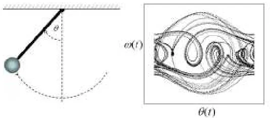
Complex behaviour (dynamical complexity) can arise even in simple systems with low compositional complexity. The damped, periodically driven non-linear pendulum is suited for illustrating the principles behind complex dynamics and chaotic attractors (Fig. 2). The dimensionless motion equation of the pendulum is:

d2θ dt2 +

1

q dθ

dt +sinθ=g cos(ωDt) (1)

withθ the angular position in radians, q the damping parameter, g the ampli-tude of the driving force, andωDthe frequency of that force. For small angleθ the

equation can be integrated, i.e. the pendulum either undergoes regular oscillations or, without a driving term, eventually stop swinging. For larger angles θ, how-ever, this approximation is invalid and hence the equation can no longer be solved analytically.

The dynamical variables of the system, i.e. the angular positionθ and velocity

ω =dθ/dt, are the coordinates defining the system’s phase space. In the two–

dimensional case, the variables can be plotted to display a phase portrait of the dynamical behaviour.

By varying the parameters q, g and ωD of the motion equation (1) and then

plotting the resulting phase portrait a wide range of behaviour can be observed. In the case of a non-zero damping parameter and no driving force to replace the energy loss, the pendulum is a dissipative system, i.e. it comes to the resting point (0,0), a fixpoint attractor. Using a non-zero driving force g, the attractor is no longer a single point at (0,0) but now a closed orbit, that is, the pendulum undergoes regular motion. A bifurcation has occurred, changing the fixpoint into a limit cycle attractor. Increasing the driving force g further, a sequence of period doublings occurs which continues as g is increased until a point is reached where the motion of the pendulum ceases to be regular and becomes chaotic, i.e. a chaotic attractor occurred.

This example nicely shows that even in a compositionally very simple system the dynamics can be chaotic. In this case, the analysis could be made because the dynamical system model, i.e. the equation of motion (1), is known.

4.3 Nonlinear time series analysis

Nonlinear time series analysis proceeds as follows: (i) reconstruction of the systems dynamics in state space; (ii) characterization of the reconstructed attractor; (iii) checking the validity of the procedure [17].

State space reconstruction. In order to reconstruct the state space using a time

series, it is resolved into coordinate values of a d-dimensional embedding space by an embedding method. Let the state space be characterized by the set of variables,

{x0(t),x1(t), ...,xd−1(t)}. Most frequently used is time delay embedding. Assume

that only time series x0(t)is available2. Then time-delayed values of this series are

used,

{x0(t),x0(t+τ), ...,x0[t+ (d−1)τ]}.

This set is topologically equivalent to the original set of system variables, see [18]. These variables are obtained by shifting the original time series by a fixed time lagτ =m∆t where m is an integer and∆t is the interval between successive

samplings. A most important problem of state space reconstruction is the determi-nation of the delay timeτand embedding dimension d for which several methods are available. This result is known as Taken’s famous ‘Embedding Theorem’ which says: valuable information about the dynamics of the system can be obtained, even if direct access to all the systems variables is impossible, as it is common in cogni-tive neuroscience!

Characterization of the reconstructed attractor. After reconstruction of the

attractor by embedding the next step is to characterize it. A common way to do this is to visualize it with a phase portrait. A phase portrait is a two– or three– dimensional plot of the reconstructed state space and the attractor. The graph shown in Fig. 1 is an example of a two–dimensional phase portrait. Other methods to display the reconstructed trajectories are Poincar´e sections and recurrence plots [19].

Following embedding and visualization of the reconstructed attractor the next step is to attempt to characterize it in a quantitative way. The classic measures applied are correlation dimension, Lyapunov exponents and entropy mentioned in Section 4, and new measures introduced frequently in the literature.

Checking the validity of the procedure. The interpretation of nonlinear

mea-sures is known to present problems sometimes since noisy time series can give rise to the unwarranted impression of low–dimensional dynamics and chaos. There-fore, the nonlinearity of the time series should be tested. It is customary to do this by surrogate data test. The null hypothesis of the test is that the original time se-ries is generated from a linear stochastic process (possibly undergoing a nonlinear static transform). Demonstration of nonlinearity is important since only nonlinear dynamical systems can have attractors other than a trivial fixpoint attractor. Chaos in particular can only occur in nonlinear dynamical systems.

2_x

5

Explanation by nonlinear dynamic analysis

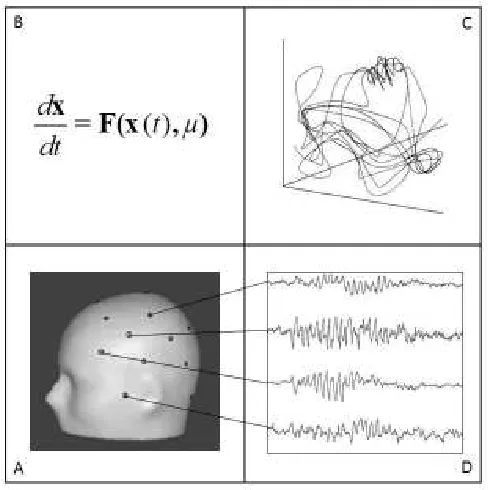
In the preceding sections the methodology of nonlinear dynamic analysis was out-lined roughly. We are now prepared to demonstrate how it is used in cognitive neuroscience. Let us consider the situation presented in Fig. 2. In cell A the phys-ical system under study is displayed (a human’s head with EEG recording sites). Cell B shows a formal model (a system of nonlinear differential equations). Estab-lishing the model requires that all the variables determining the system and their dynamic connections are exactly known. In cell C the phase portrait in the system state space is schematically illustrated. It allows to describe the possible system behaviour in terms of trajectories, attractors, bifurcations etc. Cell D presents the observed system behaviour which is often measured in cognitive science in the form of time series (in this case the EEG activity recorded via several channels).

Figure 2: Reductionist, deductive explanation is illustrated by following the path through cells A→B→C→D. This approach fails in non-decomposable systems

with complex dynamics since no system equations can be established. Instead, ob-servable behaviour of the real system is explained by nonlinear dynamic analysis, i.e. move C→D is to be made (inspired by [16]).

physical system as measured at the emergent level is reduced via the formal model to the lower level of the physical substrate. The transitions between the fields are all non-trivial. Move A→B requires to determine the relevant system

vari-ables and to study their dynamics which is rather unfeasible in the case of neuro-cognitive systems. Move B→C means nonlinear dynamical analysis of system

equations which may pose serious difficulties, depending on system characteris-tics. Finally, by moving C→D the formal constructs of nonlinear system theory

are to be mapped on real, observable phenomena in the neuro-cognitive system. This move again is very challenging, and cannot be formalised [12].

Emergent phenomena of the real, dynamically complex system must be ex-plained using nonlinear dynamic analysis since traditional analyses fail. That is, in the scheme of Fig. 2 only move C→D is (and can be) made. A meanwhile

fa-mous example is the work by Babloyantz and Destexhe [15] who demonstrated that the epileptic electric brain activity measured by the EEG forms a chaotic attractor. Here the Lyapunov exponents of the attractors and the embedding dimension of the phase space was calculated from the time series of the EEG. This was done with-out having available a formal model. From the mere fact that a chaotic attractor with certain mathematical properties is present, non-trivial conclusions (e.g., on stability, dimensionality of embedding space etc.) has been drawn.

Systemic explanations of this kind have explanatory power because dynami-cally complex systems own certain universal properties. If a whole class of dy-namic systems is characterised by a certain qualitative property, it is unnecessary to know the exact form of the special dynamic model which explains the particular emergent phenomenon. It is only necessary to assure that the system under study belongs to the corresponding class of dynamic systems in which certain qualitative phenomena are universal. This kind of the explanation works because classes of dynamically complex systems own qualitative properties (attractor types, bifurca-tions, pattern generation, chaos).

6

Conclusions

The progress made with analyses of compositionally complex (complicated) sys-tems such as artificial neural networks, cellular automata etc. has led many to believe that this can be achieved with dynamically complex systems, too. This means that the reverse engineering method has to be applied to the observed dy-namically complex phenomenon to work out which mechanism explains it best. A mechanism is known if the participating system components and their interactions are known, i.e. the term ‘mechanism’ is nearly synonymous with ‘decomposabil-ity’. If we remember that dynamically complex systems are not decomposable, it follows that no mechanism can be revealed, and the reductionist analysis fails!

expla-nations when they are complemented by a formal model and by the physical basis of the empirical system. However, this view again ignores the specificity of the dynamically complex systems which do not allow reductionist, mechanistic expla-nation. Thus, nonlinear dynamic analyses provide full-value explanations which are highly appropriate to the situation in cognitive neuroscience.

References

[1] Schierwagen, A.: Brain complexity: analysis, models and limits of under-standing. In: J. Mira et al. (Eds.): IWINAC 2009, Part I, LNCS 5601, Springer-Verlag Berlin Heidelberg, pp. 195-204 (2009)

[2] Schierwagen, A.: On reverse engineering in the cognitive and brain sciences. Natural Comput. (2011) in press

[3] Systems of Neuromorphic Adaptive Plastic Scalable Electronics (SyNAPSE). DARPA / IBM (2008)

[4] Markram, H.: The Blue Brain Project. Nature Rev. Neurosci. 7 (2006) 153– 160

[5] de Garis, H. et al.: The China-Brain Project: Building China’s Artificial Brain Using an Evolved Neural Net Module Approach. In: Pei Wang, Ben Goertzel, and Stan Franklin (Eds.): Proceedings First AGI Conference, IOS Press, Am-sterdam, The Netherlands, pp. 107–121 (2008)

[6] de Garis, H., Shuoa, C., Goertzel, B., Ruiting, L.: A world survey of artificial brain projects, Part I: Large-scale brain simulations. Neurocomput. 74 (2010) 3–29

[7] Goertzel, B., Ruiting, L., Arel, I., de Garis, H., Chen, S.: World survey of artificial brains, Part II: Biologically inspired cognitive architectures. Neuro-comput. 74 (2010), 30–49

[8] Edmonds, B.: Syntactic Measures of Complexity. PhD thesis, University of Manchester (1999)

[9] Chu, D., Strand, R., Fjelland, R.: Theories of complexity. Complexity 8 (2003) 19–30

[10] Gershenson, C.: Complexity. arXiv:1003.5947v1 [nlin.AO]

[11] Editorial. Complicated is not complex. Nature Biotechnology 17 (1999) 511

[13] Rosen, R.: Essays on Life Itself. Columbia University Press, New York (2000)

[14] Kitto, K.: High End Complexity. Intern. J. Gen. Syst. 37 (2008) 689–714

[15] Babloyantz, A., Destexhe, A.: Low-dimensional chaos in an instance of epilepsy. Proc. Natl. Acad. Sci. USA, 83 (1986) 3513–3517

[16] Jaeger, H.: Dynamische Systeme in der Kognitionswissenschaft. Kognition-swissenschaft 5 (1996) 151–174

[17] Stam, C.J.: Nonlinear dynamical analysis of EEG and MEG: Review of an emerging field. Clin. Neurophysiol. 116 (2005) 2266-2301

[18] Takens, F.: Detecting strange attractors in turbulence. Lecture Notes Math., Vol. 898, pp. 366–381 (1981)