Increased Proportion of Variance Explained and Prediction Accuracy of Survival of Breast Cancer Patients with Use of Whole-Genome Multiomic Profiles

(1)

HIGHLIGHTED ARTICLE | GENOMIC SELECTION

Increased Proportion of Variance Explained and

Prediction Accuracy of Survival of Breast Cancer

Patients with Use of Whole-Genome

Multiomic Pro

ﬁ

les

Ana I. Vazquez,*,1_{Yogasudha Veturi,}†_{Michael Behring,}‡,§_{Sadeep Shrestha,}§_{Matias Kirst,**},††

Marcio F. R. Resende, Jr.,**,††_{and Gustavo de los Campos*},‡‡

*Department of Epidemiology and Biostatistics, Michigan State University, East Lansing, Michigan 48824,†Biostatistics

Department,‡Comprehensive Cancer Center, and§Department of Epidemiology, University of Alabama at Birmingham, Alabama

35294, **School of Forest Resources and Conservation and††University of Florida Genetics Institute, University of Florida,

Gainesville, Florida 32611, and‡‡Statistics Department, Michigan State University, East Lansing, Michigan 48824

ABSTRACTWhole-genome multiomic proﬁles hold valuable information for the analysis and prediction of disease risk and progression.

However, integrating high-dimensional multilayer omic data into risk-assessment models is statistically and computationally challenging. We describe a statistical framework, the Bayesian generalized additive model ((BGAM), and present software for integrating multilayer high-dimensional inputs into risk-assessment models. We used BGAM and data from The Cancer Genome Atlas for the analysis and prediction of survival after diagnosis of breast cancer. We developed a sequence of studies to (1) compare predictions based on single omics with those based on clinical covariates commonly used for the assessment of breast cancer patients (COV), (2) evaluate the benefits of combining COV and omics, (3) compare models based on (a) COV and gene expression profiles from oncogenes with (b) COV and whole-genome gene expression (WGGE) profiles, and (4) evaluate the impacts of combining multiple omics and their interactions. We report that (1) WGGE profiles and whole-genome methylation (METH) profiles offer more predictive power than any of the COV commonly used in clinical practice (e.g., subtype and stage), (2) adding WGGE or METH profiles to COV increases prediction accuracy, (3) the predictive power of WGGE profiles is considerably higher than that based on expression from large-effect oncogenes, and (4) the gain in prediction accuracy when combining multiple omics is consistent. Our results show the feasibility of omic integration and highlight the importance of WGGE and METH profiles in breast cancer, achieving gains of up to 7 points area under the curve (AUC) over the COV in some cases.

KEYWORDSprediction of complex traits; diseases risk; omics integration; GenPred; Shared data resource; genomic selection

T

HE continued development of high-throughput genomic

technologies has fundamentally changed the genetic analyses of complex traits and diseases. These technologies

provide large volumes of data from multiple“omic”layers,

including the genome (e.g., SNPs, copy-number variants,

and mutations), the epigenome (e.g., methylation), the

transcriptome (e.g., RNA-seq), the proteome, and so on.

This information can be used to develop models for under-standing and predicting disease risk and disease prognosis. Recently, several studies have uncovered unprecedented numbers of omic factors associated with disease risk and progression. For instance, in the last decade, genome-wide association studies (GWAS) have reported large numbers

of SNPs (e.g.,http://www.genome.gov/gwastudies/) and

structural variants [e.g., copy-number variants (Beroukhim

et al. 2010; Morrow 2010)] associated with disease risk. Likewise, several studies have reported methylation sites

(Dedeurwaerderet al.2011; Fackleret al.2011; Fanget al.

2011) and genes with expression proﬁles associated with

prognosis (Perouet al.2000; Sørlieet al.2001; Van’t Veer

Manuscript received November 22, 2015; accepted for publication April 12, 2015; published Early Online April 27, 2016.

Available freely online through the author-supported open access option.

Supplemental material is available online atwww.genetics.org/lookup/suppl/doi:10. 1534/genetics.115.185181/-/DC1.

(2)

et al.2002; Sotiriou and Pusztai 2009; Gyorffyet al.2016). However, despite the tremendous progress achieved, use of this information in clinical practice remains limited in part because the proportion of variance in disease risk or prognosis explained

by the individual factors identiﬁed still remains limited.

Data integration can be an avenue for improving our un-derstanding and our ability to predict disease risk and prog-nosis. Integration can take place by combining information from multiple sites across the genome as well as by integrat-ing inputs from different omics. In prediction of complex

traits and disease risk, several studies (e.g., Purcellet al.2009;

de los Camposet al.2010c; Yanget al.2010; Makowskyet al.

2011; Vazquezet al.2012) have demonstrated that the

pro-portion of variance explained by use of whole-DNA proﬁles is

considerably higher than that achieved by models that use a

limited number of GWAS-signiﬁcant variants. Likewise, several

studies have demonstrated beneﬁts of integrating data from

multiple omics. For example, Chenet al.(2012) demonstrated

how integrated omic proﬁles can provide insights into the

de-velopment of type 2 diabetes. However, our ability to integrate whole-genome multilayer omic data into risk assessments still lags behind.

Wheeleret al.(2014) and Vazquezet al.(2014) proposed

using what Wheeler called “Omic Kriging” for prediction

of complex traits and disease risk using multiomic proﬁles.

Kriging is a kernel-smoothing technique commonly used in

spatial statistics (e.g., Cressie 2015). From a statistical

per-spective, kriging is the best linear unbiased predictor (BLUP) method commonly used in quantitative genetics (Henderson 1950; Robinson 1991) using pedigree (Henderson 1950, 1975) or DNA information (G-BLUP) (VanRaden 2008)].

OmicKriging is a multikernel method (de los Camposet al.

2010a, b) in which the resulting kernel is a weighted average of similarity matrices derived from different omics.

Although OmicKriging represents a promising method for integrating multiomic data, the method has potentially important limitations. First, the approach assumes that the architecture of effects is homogeneous across omic layers. This assumption may not hold if some omics have a sparse

architec-ture of effect (i.e., a few factors have sizable effects, and the rest

have no effect) and other omics have non-sparse-effects

archi-tecture (i.e., all inputs have small effects). Second, OmicKriging

assumes implicitly that omics act in an additive manner (i.e.,

there are no interactions between omics). This may fail, for

instance, if the effects of one layer (e.g., SNP) are modulated

by a second layer (e.g., methylation).

In this study, we describe a modeling framework that (1) allows integration of high-dimension inputs from multiple omic layers, (2) contemplates different effect architectures across layers, and (3) incorporates interactions between omics. The approach is a Bayesian generalized additive model

(BGAM) that integrates in a uniﬁed setting ideas from

general-ized additive models (Hastie and Tibshirani 1986) with Bayesian methods that allow for different architectures of effects (includ-ing estimation with or without shrinkage and variable selection methods) and recently developed techniques for modeling

interactions between high-dimensional inputs (Jarquín et al.

2014). Importantly, the BGAM can be used with traditional quantitative traits and time-event (subject to censoring),

ordi-nal, and binary (e.g., disease) outcomes.

We use BGAM and data from The Cancer Genome Atlas (TCGA) to develop models for analysis and prediction of breast cancer (BC) outcomes. Breast cancer is considered one of the most lethal types of cancer (Boyle and Levin

2008). In the United States alone, there are180,000 new

cases of BC each year (Eifel et al. 2000), and it has been

estimated that about 12% of women will develop BC over

their lifetime (Eifelet al.2000; Smigalet al.2006). Advances

in early detection and in adjuvant therapy have reduced mor-tality due to BC. However, adjuvant therapy has important undesirable side effects on treated patients. Some of the most serious ones include permanent infertility, heart damage, cognitive impairment, and increased probability of developing

other types of cancers (Eifelet al. 2000). Cancers in

approxi-mately 40% of BC patients are estimated to recur or metastasize

(Weigeltet al.2005). However, because current models cannot

accurately predict BC progression, approximately 80% of BC patients are treated with adjuvant therapy. Thus, a substantial number of BC patients are being treated unnecessarily with adjuvant therapy. An accurate assessment of disease progres-sion could be used to implement a more precise approach to the treatment of BC patients and reduce the impact of undesirable outcomes due to therapy. Here we apply a BGAM modeling framework to data from TCGA to develop models for prediction of the probability of survival after a diagnosis of BC. In our application, we compare multiomic models with risk

assess-ments based on clinical covariates and the expression proﬁles

of large-effect genes included in the Oncotype DX platform

(Genomic Health) (Paik et al.2004, 2006), which is a Food

and Drug Administration (FDA)–approved platform used in

clinical practice to predict BC progression. Our analysis

demon-strates that the integration of whole-omic proﬁles can increase

the proportion of interindividual differences in survival and enhance prediction accuracy of BC outcomes above and beyond

that which can be achieved using clinical covariates (i.e., race,

age, cancer subtype, and stage) and expression-based

diagnos-tic tools (e.g., Oncotype DX).

In this article, we outline the main elements of the BGAM modeling framework and present a series of case studies in which we apply the methods to BC cases from TCGA. The

Discussionsection highlights the mainﬁndings of our study and offers a brief perspective on the strengths and limitations of the BGAM framework. Our results show how the integra-tion of omics in a clinical model improves predicintegra-tion accuracy for most omics, but the improvements are higher by combin-ing clinical information with whole-genome methylation and

gene expression proﬁles.

Modeling Framework

Assume that the multilayer omic data consist of a phenotype or

(3)

coming fromLinput layers; these layers may include demo-graphics, clinical covariates, and data from several omics. We

denote the data from these layers asX¼ fX1;. . .;XLg. Here

Xl¼ fxlijgdenotes a set of predictors from thelth data layer,

andl =1,. . .,L,i =1,. . .,n, andj =1,. . ., plindex input

layersl, individualsi, and predictors within an input layerj,

respectively.

Generalized additive model (GAM)

Multilayer inputs can be incorporated into a regression model using the so-called generalized additive model (GAM) frame-work (Hastie and Tibshirani 1986). In a GAM, a regression

function is expressed as the sum ofLsmooth functions

hi¼f1ðX1i;a1Þ þf2ðX2i;a2Þ þ⋯þfLðXLi;a1Þ (1)

Each of these functions can be linear or nonlinear for the

inputs and can be speciﬁed parametrically or using

semi-parametric methods (e.g., splines). Typically, these

func-tions are indexed by a set of parametersalestimated from

data. When these parameters are high dimensional (i.e.,plis

large), estimation is typically carried out using L2-penalized

(i.e., ridge-regression) estimators (Hastie and Tibshirani 1986);

this approach renders smooth functions with shrunken param-eter estimates. The extent of shrinkage of estimates is controlled by regularization parameters. When there is only smooth func-tion, an optimal value for the regularization parameter can be

chosen using cross-validation methods (e.g., Golubet al.1979).

However, when there are multiple regularization parameters

(e.g., one per term of the linear predictor), the cross-validation

approach becomes infeasible, and other approaches (e.g.,

mixed-effects models or Bayesian methods) are needed.

For some high-dimensional inputs (e.g., DNA markers and

transcriptomes), variable selection, as opposed to shrinkage, may be desirable. This can be achieved in penalized regressions

by using penalties other than those based on the L2 norm,e.g.,

with the L1 norm, as in the LASSO method (Tibshirani 1996). Alternatively, variable selection and/or shrinkage can be obtained in a Bayesian setting by choosing particular types of prior distri-butions. The Bayesian approach has several attractive features. First, within a Bayesian framework, multiple regularization pa-rameters can be estimated from data without the need to conduct extensive cross-validations. Second, Bayesian mod-els can accommodate both shrinkage and variable selection

in a uniﬁed framework. Finally, using methods described later,

within the Bayesian framework, one can accommodate in-teractions between inputs in high-dimensional sets. There-fore, in this study, we adopted a Bayesian generalized additive model (BGAM) framework for integrating multiomic inputs.

Bayesian generalized additive model (BGAM)

For ease of presentation, we introduce the model for the case of a Gaussian outcome and assume that each of the functions entering in (1) are linear on their inputs. Cases involving non-Gaussian outcomes or functions that are nonlinear on inputs are considered later. For the purpose of illustration,

we consider only three input layers, including a set of

nongenetic covariates X1i¼ fx1ijgj_j¼_¼p₁1 and two omics

X2i¼ fx2ijg j¼p₂

j¼1 andX3i ¼ fx3ijg j¼p₃

j¼1 . Extensions to more than

three layers are straightforward. With this setting, the lin-ear predictor becomes

hi¼mþ X j¼p1

j¼1

x1ija1jþ X j¼p2

j¼1

x2ija2jþ X j¼p3

j¼1

x3ija3j (2)

wherea1¼ fa1jgjj¼¼p11,a2¼ fa2jgjj¼¼p12, anda3¼ fa3jgjj¼¼p13 are

regression coefﬁcients.

Bayesian likelihood

Under Gaussian assumptions, the conditional distribution of the outcome given the parameters of the linear predictors is

pðyjX1;X2;X3;uÞ ¼ Y i¼n

i¼1

Exp

2ðyi2hiÞ 2

2s2 e

ffiffiffiffiffiffiffiffiffiffiffiffi

2ps2

e

p (3)

where u¼ fs2

e;m; a1;a2;a3g is a vector of model

unknowns.

Prior distribution

In a Bayesian setting, layer-speciﬁc architectures of effects can

be accommodated using layer-speciﬁc priors. Therefore, we

structure the joint prior distribution of effects as follows:

pa1;a2;a3;s2_e;V1;V2;V3

}p

s2 e

Y3

l¼1

" Y

j¼pl

j¼1

pðaljjVlÞ

# pðVlÞ

where pðs2

eÞ is a prior for the error variance (e.g., a scaled

inverse chi-square),pðaljjVl Þare IID priors assigned to the

effect of the1st input layer,Vlis a set of layer-speciﬁc

regu-larization hyperparameters, andpðVlÞis a prior distribution

assigned to these hyperparameters.

Special cases

Estimation without shrinkage can be obtained by setting

pðaljjVl Þ to be aﬂat prior (e.g., a normal prior centered

at zero and with a very large variance). Shrunken estimates

can be obtained by setting pðaljjVl Þto be a normal prior

centered at zero and with variance parameter (Vl¼s2_a_l)

treated as unknown. This approach renders estimates

com-parable to those of ridge regression (Meuwissenet al.2001)

with an extent of shrinkage that is similar across effects. Differential shrinkage of estimates of effects can be ob-tained using priors from the thick-tailed family, such as the

double-exponential or scaled-tdistributions; these priors are

used in the Bayesian LASSO (Park and Casella 2008) and

in BayesA (Meuwissenet al.2001). Finally, variable selection

can be achieved by settingpðaljjVl Þ to be aﬁnite mixture

with a point of mass (or a very sharp spike) at zero and a

relativelyﬂat slab (George and McCulloch 1993; Ishwaran

(4)

Functions that are nonlinear inputs

These can be accommodated by ﬁrst mapping the original

inputs (e.g.,Xl) into a set of basis functionsFl¼ ffl1ðXlÞ;

fl2ðXlÞ;. . .gand then using the transformed inputsfljðXlÞas

covariates in the regression. This can be done either in

para-metric settings (e.g., with polynomials) or with

semiparamet-ric speciﬁcations (e.g., using splines or kernels).

Gaussian processes

When the coefﬁcients entering a linear term are assigned IID

normal priors, the resulting function can be viewed as a draw

from a Gaussian process. For instance, ifalj Nð0;s2_a_lÞ, then

the functionfl¼Flalfollows a normal distribution with null

mean and covariance matrix given byKls2_a_l, whereKl¼FlF9l

is a covariance structure computed using cross-products of the basis functions. This treatment fully connects the BGAM with reproducing kernel Hilbert spaces (RKHS) regression methods (Wahba 1990; Shawe-Taylor and Cristianini 2004), a framework that can be used to implement various types of parametric and semiparametric regressions. Importantly, this framework can be implemented with almost any input sets, including text data, images, special data, graphs, and so on

(Wahba 1990; de los Camposet al.2009, 2010a).

Interactions between input layers

Model of expressions (1) and (2) assume that layers act additively. However, many applications may require modeling interactions between layers. Accommodating interactions can be particularly challenging when the number of inputs in the interacting layers is large. For instance, with 10,000

expres-sion proﬁles and 10,000 SNPs, modeling all possibleﬁrst-order

interactions requires using 100 million contrasts. Dealing with interactions explicitly is not feasible. Therefore, we propose to deal with interactions implicitly using Gaussian processes with covariance structures based on the patterns induced by the so-called reaction-norm model. This approach has been used for modeling interactions between genetic factors and environmental covariates in plants and animals (Gregorius

and Namkoong 1986; Calus et al. 2002; Su et al. 2006;

Jarquínet al.2014). Recently, Jarquínet al.(2014) developed

methods for reaction norms involving high-dimensional

ge-netic (e.g., SNP) and high-dimensional environmental inputs.

The authors show that the covariance patterns induced by a reaction-norm model can be expressed as the Schur (or Hadamard) product of kernels that evaluate input similarity at each of the interacting layers. An example of the use of this method is provided in the fourth case study of the next section.

Non-Gaussian outcomes

Non-Gaussian outcomes (e.g., binary or ordered categorical

outcomes) can be accommodated using the probit or logit link; in a Bayesian Markov chain Monte Carlo (MCMC) set-ting, the probit link can be implemented easily using data augmentation (Albert and Chib 1993).

Software

All the models described in this section can be implemented using the Bayesian generalized linear regression (BGLR) R package (Pérez and de los Campos 2014). This software im-plements BGAM for continuous, binary, and ordinal outcomes and offers users the possibility of specifying at each of the layers parametric and semiparametric methods for shrinkage and variable selection. Further details about the software can be found in Pérez and de los Campos (2014) and at the

following website:https://github.com/gdlc/BGLR-R/.

Case Studies

In this section, we investigate the association between patient survival and several predictors that can be assessed at di-agnosis, including information commonly used by clinicians to assess BC patients (hereafter we refer to these predictors as

“clinical covariates”), gene expression proﬁles (RNA-seq),

methylation, copy-number variant, and micro-RNA. All these omics were assessed at the primary tumor. We consider sev-eral research questions, and for each of these questions, we designed a case study that involves the comparison of several models, each of which is a special case of the BGAM frame-work described in the preceding section. All the case studies are based on data from BC patients from TCGA. The

motiva-tion for each of the case studies is brieﬂy presented next.

Case study I

Clinical information such as tumor subtype or cancer stage is used to assess risk of possible cancer outcomes; precise pre-diction of outcomes improves the decision as to which treat-ment options should be used for each patient. Although the clinical covariates are predictive of the likelihood of disease progression, after accounting for differences attributable to these clinical predictors, important interindividual differences in the BC outcome remain. Gene expression has been

dem-onstrated to be associated with BC progression (Sørlieet al.

2001, 2003). Therefore, in our ﬁrst case study (CS-I), we

assessed the relative contribution to variance and prediction

accuracy of whole-genome gene expression (WGGE) proﬁles.

We compare models based on WGGE proﬁles with others

based on clinical covariates commonly used in clinical prac-tice (BC subtype, stage, age at cancer diagnosis, histologic subtype, and race). In this study, we assessed the contribution

to variance and prediction accuracy of WGGE proﬁles alone

and in combination with clinical covariates. Sørlie et al.

(2001) demonstrated that clusters derived from the gene

expression proﬁles are associated with breast cancer

sub-types. Our COV (M7) model and all other models that in-corporate all clinical covariates already accounts for BC subtypes as dummy variables and therefore incorporates clustering. Several studies have demonstrated the association of gene expression patterns and BC outcome. However, these studies are based on data that have been conditioned by some

(5)

components). We argue that consideration of WGGE proﬁles is essential in capturing the diverse information on this trait of complex biology.

Case study II

Ourﬁrst case study accounted for the main effects of

com-monly used clinical covariates and those of WGGE proﬁles.

However, the patterns of gene expression and the prognosis of the cancer present substantial variation in both the dif-ferent cancer subtypes and the difdif-ferent stages of devel-opment of the disease. Therefore, in our second case study (CS-II), we focused on a particular cancer subtype: luminal

types at early stage—this is the most prevalent subtype.

For early-stage luminal patients, there is a well-established commercial gene expression platform (Oncotype DX;

Geno-mic Health, Inc, Redwood City, CA) (Paiket al.2004, 2006)

that has been approved by the FDA for use as a diagnostic

tool. Oncotype DX analysis is based on the proﬁle of a genetic

signature consisting of only a few genes. We argue that the

use of whole-genome gene expression proﬁles can lead to a

larger proportion of variance explained and higher prediction

accuracy than can be achieved using the expression proﬁles

of a few genes. Therefore, in CS-II, we compared models based on (1) clinical covariates, (2) clinical covariates plus

the expression proﬁle of genes included in the Oncotype DX,

and (3) clinical covariates and WGGE proﬁles. The models

wereﬁtted and compared based on data from patients with

luminal types at early stage only, lymph node negative, and all lymph nodes.

Case study III

Information from omics other than the transcriptome, such as

DNA information (e.g., copy-number variants), or data from

the epigenome also can contribute to interindividual differ-ences in survival. Therefore, in our third case study (CS-III), we considered the use of omics other than WGGE

pro-ﬁles, including micro-RNA (miRNA), methylation, and

copy-number variant (CNV). For each omic, we assessed the proportion of variance explained and prediction accuracy of the omic alone and in conjunction with clinical covariates; in all cases, we considered one omic at a time and conducted separate analyses for each of the omics.

Case study IV

In our previous case studies, we assessed omics separately or in combination with COV. In our fourth case study (CS-IV),

we evaluated the beneﬁts of integrating two omics, WGGE

and METH proﬁles and COV simultaneously; we explored

this both with an additive model and with a speciﬁcation

that contemplates interactions between omics.

Data

The Cancer Genome Atlas (TCGA) offers data on BC patients with demographic, clinical, omic, and follow-up information from which survival information can be derived. Because data are still being collected, follow-up time is short for most

patients. Therefore, our response variable was deﬁned as

subjects that either died (1) or were alive (0) and had at least three years of follow-up. All male records and females with

incomplete follow-up or inconsistent clinical records (e.g.,

death shortly after the diagnosis of BC in an early stage with-out any record of progression) were removed. Also, women with distant metastases at the time of diagnosis or patients with history of a previous cancer were removed. After editing, these samples were reduced from over 1000 to 797 samples, from which only 285 met the minimum follow-up criteria. Thus, the baseline data set consisted of 285 patients; these included subjects with concordant data that were either dead

(n= 60) or alive (n= 225) and had a minimum follow-up

time of 3 years. Not all these patients had complete data for all the omics. Therefore, in some of the case studies, we further narrowed the set of patients to those who had

com-plete data for the inputs relevant to the speciﬁc analysis. The

original data set offered by TCGA was reduced to patients with at least three years of follow-up because follow-up is still too short [in the original TCGA data, the follow-up time

averages (6SD) 2.05 (61.14) years of last contact time for

those still alive.]

In CS-I, CS-III, and CA-IV, models were obtained by regressing alive status (0/1) on the inputs that follow. These inputs were selected based on their association with survival in preliminary analyses. CS-II is a more homogeneous

pop-ulation, and fewer covariables were used (seeCase study II

section).

Demographics: Demographics included age at diagnosis

[55.6 6 12.6 years (mean 6 SD)] and race/ethnicity

(Caucasian/African American).

Clinical information from the tumor: Tumor clinical in-formation included histologic type [whether the invasive

tumor arose from lobular tissue (n= 35) or from ductal

breast tissue (n= 251)], subtype classiﬁcation based on

the membrane receptors present in the tumor cell (luminal A, 179; luminal B, 24; Her2-Neu, 69; and triple negative, 13),

and stage, as deﬁned by the American Joint Committee on

Cancer (Edgeet al.2010) (from I–IV; the number of patients

per stage were 58, 159, and 68 in stages I, II, and higher, respectively).

Omics data: Omics data included gene expression

pro-ﬁles from RNA-seq, whole-genome methylation, miRNA, and

CNVs. Gene expression proﬁles were assessed using RNA-seq

technology sequenced on an Illumina HiSeq 2000 platform.

Normalized expression counts per gene were used. Workﬂows

for the creation of level 3 RNA data were detailed

previ-ously (Liet al.2010; Wanget al.2010). CNV data were

de-rived from Affymetrix Genome-Wide SNP Array 6.0. Mean

log2ratios were used as a measure of per-segment CNVs.

Full processing details are documented in a Broad Institute

GenePattern pipeline (“GenePattern”). Source data for

(6)

HumanMethylation450 Beadchip and were processed by the Johns Hopkins GSC to derive beta values for CpG sites and their association with gene regions using methylumi

(Pidsley et al. 2013). miRNA values are quantiﬁed as

reads per million (RPM) from the Illumina HiSeq miRNA 2500 platform. Short-sequence reads were aligned to the RCh37-lite reference genome using the Burrows-Wheeler Alignment (BWA) tool (Li and Durbin 2009) and normal-ized as RPMs (Network 2012). In TCGA, samples were randomly assigned to plates; therefore, there should be no association between batch and survival outcomes.

However, to conﬁrm this, we conducted analyses of

dis-persion due to batch (see Supplemental Material,File S1,

Table S1.1).

Data analysis

Each of the case studies includes a baseline model plus extensions obtained by including different combinations of omics. In all cases, the response (survival, Yes/No) was regressed on predictors using a threshold model (Gianola and Foulley 1983; Agresti 2012) as implemented in the BGLR R package (Pérez and de los Campos 2014). In each study,

models wereﬁrstﬁtted to all the individuals that had

com-plete data for the set of predictors used in the case study.

From this analysis, we reported parameter estimates (e.g.,

variance components) and the posterior means of the log likelihoods.

Model speciﬁcation: The effects of clinical covariates were

regarded as ﬁxed, while the effects of different omics

were regarded as random. For simplicity, all random effects

were assumed to be IID Gaussian, with omic-speciﬁc variance

parameters. We also conducted analyses using priors that induce variable selection. In other studies, these models did

not show strong differences in risk for disease (Vazquezet al.

2015). Results of these analyses are given in the File S1,

Table S1.2. Variance parameters were assigned scaled

in-verse-chi-square priors with ﬁve degrees of freedom (this

gives a weakly informative prior) and scale parameters com-puted according to the rules described in Perez and de los Campos (2014); this is the default treatment of variances implemented in BGLR. For each model, we ran 500,000

iter-ations of a Gibbs sampler; theﬁrst 20,000 samples were

dis-carded as burn-in, and the remaining samples were thinned

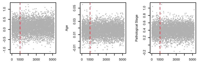
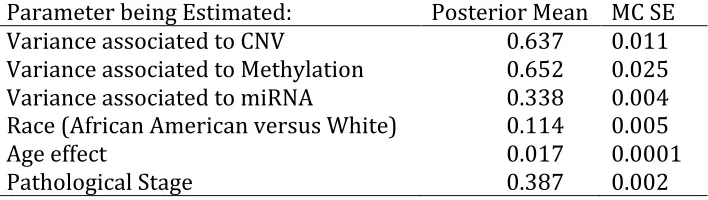
at a thinning interval of ﬁve (seeFile S1, Figure S1.1 and

Figure S1.2 and Table S1.3). For all case studies, we report the log likelihood, effective number of parameters in the model, and the deviance information criteria (DIC).

Prediction accuracy: Prediction accuracy was assessed us-ing cross-validations (CVs). We implemented a total of 200 independently generated 10-fold CVs. Prediction accuracy was

assessed using the CV–area under the receiver operating

char-acteristic curve (CV-AUC) (e.g., Fawcett 2006). Therefore, for

each study and model, we had a total of 200 estimates of CV-AUC. Models were compared based on the average CV-AUC

and also by counting the proportion of CVs (of 200) for which a given model had a higher CV-AUC than another. For CV

analyses, models wereﬁtted using 80,000 iterations collected

after discarding the ﬁrst 15,000 samples; furthermore,

sam-ples were thinned at an interval ofﬁve. For all case studies, we

report the average and SD (across 200 CVs) of the CV-AUC and the proportion of times that a model had a CV-AUC greater than other models, also computed using results from 200 CVs. Code to implement the models described herein is provided in

File S2 and on the following website: https://github.com/ anainesvs/VAZQUEZ_etal_GENETICS_2016.

Data availability

The data used in this study is publically available, collected and distributed by TCGA, National Institutes of Health/National

Cancer Institute project. Data can be obtained at

https://tcga-data.nci.nih.gov/tcga. Additionally, to ensure reproducibility of this analysis, the lines of code used to execute this study

are provided in File S2 and at the above- mentioned github

repository.

Results

Case study I: integrating clinical covariates and whole-genome gene expression

Theﬁrst case study (CS-I) was designed to assess the

mar-ginal association between survival and individual risk

fac-tors composed of clinical covariates (e.g., age, race, etc.) and to

quantify the gains in prediction accuracy that can be achieved by adding gene expression data on a model that accounts for the clinical information. Six sets of risk factors were consid-ered; these included two demographics (age and race), three clinical features of the cancer (whether it is a lobular carci-noma, cancer subtype, and pathologic stage), and gene

expres-sion proﬁles (RNA-seq) from the primary tumor.

Sequence of models: A total of eight models were ﬁtted,

including six single-risk-factor models (labeled as M1–M6),

a model based on all predictors except gene expression (M7, also labeled as COV), and a model that included all the avail-able predictors (M8, labeled as COV + WGGE).

Results:Table 1 provides goodness-of-ﬁt statistics, measures of model complexity, and estimates of prediction accuracy for

each of the eight models ﬁtted in CS-I. Among the

single-factor models, the one thatﬁtted the data best and had the

highest CV-AUC was the model using whole-genome gene

expression (WGGE, M6); clearly, WGGE proﬁles were the

most informative input.

Comparison of the results obtained with models COV and

COV + WGGE indicate that information from WGGE proﬁles

can improve the assessment of survival, even after accounting for the predictors commonly considered in clinical practice.

The increase in CV-AUC obtained when WGGE proﬁles were

(7)

1.7 points (COV + WGGE) higher than that for a model based on COV, and the comparison across 200 CVs shows that the model COV + WGGE outperformed the model based on clinical covariates (COV) 99% of the time. In other words, the increase in prediction accuracy was consistent.

Case study II: genetic signatures vs. whole-genome gene expression proﬁles within cancer subtypes

CS-I showed that the assessment of BC survival could be

improved by using WGGE proﬁles from the tumor tissue.

CS-I is an analysis that is not speciﬁc to a cancer subtype,

although subtypes are considered in the model. The clinical

value of WGGE proﬁles for BC has been demonstrated

pre-viously (Sørlieet al.2001), and gene expression proﬁles from

oncogenes are often used to assess BC patients; an example of

this is the Oncotype DX platform (Paik et al.2004, 2006),

which is based on the expression proﬁles of 21 genes.

Onco-type DX has been validated for assessing BC outcome among

patients affected by tumors of the luminal (estrogen receptor–

positive [ER+]) cancer subtype that are in an early stage of disease and do not have distant or nodal metastases. Therefore, in this case study, we focused only on luminal cancers and compared the relative contribution to variance and to prediction

accuracy of the expression proﬁle of the Oncotype DX with that

of WGGE proﬁles.

Data:Data consist of a subset of the patients (n= 186) used in CS-I who qualify for the Onctoype DX test; these are patients who had ER+ tumors at stage I or stage II. Results are

pre-sented for all early-stage luminal patients [ER+_or

progester-one receptor positive (PR+)] and only for early-stage luminal patients with negative lymph nodes (the target population of

the Oncotype DX). The platform includes 21 genes, 16“risk”

genes, and 5 reference (“housekeeping”) genes for the purpose

of normalizing the data (Paik et al. 2004). From RNA-seq

WGGE proﬁles, we retrieve the expression proﬁles from all

the risk genes, exceptRPLP0.

Sequence of models:The baseline model (COV) included age at diagnosis, race, and ethnicity. Tumor subtype and stage were not included as covariates of the baseline model because all patients had luminal tumors in early stage. The baseline

model wasﬁrst extended by adding the random effects of the

expression of the genes included in the Oncotype DX panel (COV + ONCO). Subsequently, we extended the COV + ONCO model by adding the random effects of 17,899 genes not included in the Oncotype DX panel (we labeled this model COV + WGGE, standing for covariates plus whole-genome gene expression). The effects of race and age were treated as

ﬁxed, and those of the gene expression proﬁles of the genes

included in either COV + ONCO or COV + WGGE were assigned IID normal priors with null mean and unknown variance (var-iances were assigned scaled inverse-chi-square priors).

Results: The results from CS-II are given in Table 2. In this study, we report CV-AUC based on luminal types, all luminals,

(8)

and only the ones with lymph node negatives. Estimates of variance components revealed that the contribution to vari-ance of the expression of the gene in the Oncotype DX was

low (0.027). However, the use of WGGE proﬁles lead to a

sizable fraction of variance explained. Indeed, the estimated

variance component associated with WGGE proﬁles (0.439)

amounts to 30% of the variance in risk that is not explained by COV (computed as 0.439/1.439). However, owing to the small sample size, the posterior credibility region for the

es-timated variance component associated with WGGE proﬁles

was wide. The DIC (“smaller is better”) also suggests that the

best model was the one including COV and WGGE proﬁles.

And the CVs based on all luminal cases revealed that adding information from the genes included in the Oncotype DX (COV + ONCO) improved CV-AUC relative to the baseline

model by 2.7 points and that adding WGGE proﬁles increased

CV-AUCs (also relative to COV) by 6.5 points. The analyses

based on patients with lymph node–negative tumors also

revealed a sizable increase in prediction CV-AUC when using

WGGE proﬁles (compared to the baseline model, the model

using COV and WGGE had 6.6 points in CV-AUC, and COV + WGGE outperformed COV in 99% of the 200 CVs). However, the prediction CV-AUC of the COV + ONCO model was sim-ilar to that obtained with the COV model only. Therefore, we

conclude that using WGGE proﬁles leads to a higher

propor-tion of variance of risk explained and a higher predicpropor-tion

accuracy than can be achieved using the expression proﬁles

of a few genes.

Case study III: comparison between omics

In the two preceding studies, we assessed the performance of models based on clinical covariates and gene expression in-formation from the tumor cells. In this study, we compared the relative performance of models based on the other omics avail-able: (1) CNVs, (2) methylation (METH), and (3) miRNA.

Data: This study includes data from patients who had in-formation for at least one of the omics considered. Figure 1 shows a Venn diagram (Oliveros 2007) representing the number of patients with omic data by layer. The number of

individuals with complete omic data are relatively small (n=

127). Therefore, when ﬁtting models for a given omic, we

used all the individuals who had information for that omic. This leads to three different sets of patients (we labeled them

as sets 1–3, corresponding to individuals with CNV, METH,

and miRNA, respectively) to which models wereﬁtted.

Sequence of models: For each set of patients, we compared the performance of a model based on covariates only (COV) with that of a model based on covariates plus data from the corresponding omic (COV + CNV, COV + METH, and COV +

miRNA). As before, models were ﬁtted using the BGLR R

package with COV as ﬁxed effects and omics as random

effects, where the effects of the omics were treated as IID drawn from a normal distribution with null mean and

un-known variance. Table

(9)

Results: Table 3 shows estimates of goodness ofﬁt, model complexity, variance components, and prediction accuracy (AUC in CV) by model. The comparison of models based on COV only with those based on one omic (either METH, CNV,

or miRNA) suggests that a model using METH proﬁlesﬁts the

data better than and predicts survival equally well (actually slightly more accurate) as a model based on COV. This

sug-gests that METH proﬁles information is capturing differences

due to tumor subtype and stage. This was not observed for models based on CNV or miRNA; in these two cases, the model based on COV outperformed the prediction accuracy of the models based on either CNV or miRNA only.

The estimates of variance components derived from models using COV plus one omic (COV + CNV, COV + METH, COV +

miRNA) show that METH proﬁles and CNVs explained a

large fraction of interindividual differences in risk that cannot be explained by COV; however, the 95% posterior credibility regions are all wide. According to DIC, the models using COV plus one omic were all better than the model using COV only; however, the differences in DIC were, relative to the model based on COV, large for the case of COV + METH and COV + CNV and very small for the model COV + miRNA (only about 2 points). Finally, the evaluation of prediction accuracy suggests

that adding either METH proﬁles or CNVs to a model based on

COV increased prediction accuracy signiﬁcantly (99% of the

time in 200 CVs) but by 1.5 to 1.7 points of AUC. Considering all the results from these case studies, it appears that among the three omics evaluated, METH was the one that explained a large proportion of variance in risk and contributed most to prediction power, both when considered alone or in combina-tion with COV.

Case study IV: integrating multiple omics

Among the four omics considered in the preceding studies, the METH and WGGE models appeared to be the ones that

explain a large proportion of variance and achieved the highest levels of prediction accuracy both when considered alone and in combination with COV. Therefore, in this case study, we considered integrating these two omics together with COV into a risk-assessment model. Furthermore, we evaluated the impacts of including interactions between the two omics using a reaction-norm model.

Data:Data include the individuals (n= 218) who had com-plete information for COV, METH, and WGGE.

Sequence of models:The baseline model (COV) is the same

as the one described in CS-I. This model wasﬁrst expanded

by adding METH and WGGE additively (COV + METH + WGGE) and subsequently further expanded by adding

in-teractions between omics (COV + METH3WGGE) using a

reaction-norm model. As before, COV was included asﬁxed

effects and omics as random effects. In all cases, the random

effects were assumed to be Gaussian, with omic-speciﬁc

vari-ance. The additive model COV + METH + WGGE had two variance parameters linked to the main effects of each of the

omics included, and COV + METH3WGGE had three

vari-ance parameters, two for main effects and one for interactions.

Results: Table 4 shows the results obtained in CS-IV. In the additive model (COV + METH + WGGE), the two omics explained about 27% of the variance in risk that was not accounted for by COV (this is estimated as the sum of the two variance components divide by the sum of the two var-iance components plus the error varvar-iance, which in the probit model is 1). When interactions were added, the estimated variance components of the main effects of each omic went down (this relative to the additive model), and the total pro-portion of variance in risk explained by omics (including main effects and interactions) stays roughly the same. The posterior mean of the log likelihood of the model COV + METH + WGGE was 15.8 points higher than that of the COV model; this indicates that adding the two omics increased

good-ness ofﬁt markedly. When interactions were added, the change

in the log-likelihood relative to COV + METH + WGGE was

more modest. DIC (“smaller is better”) indicates a clear

su-periority of the additive model with two omics relative to COV and almost no difference between COV + METH +

WGGE and COV + METH3WGGE. Finally, the evaluation of

prediction accuracy from CVs showed that (1) the baseline model had a reasonably good AUC (0.724), (2) the additive model improved the performance by 3 points in AUC (importantly, this increase happened in 99% of the 200 CV), and (3) adding inter-actions did not clearly improved prediction accuracy (in 60% of the CV the additive model was better than the model having interactions, and in the other 40%, the opposite happened).

Discussion

The availability of multiomic data sets has increased recently, and this trend is expected to continue. Modern omic data sets Figure 1 Venn diagram with the number of patients who had

(10)

can be big (largen), high dimensional (each subject can have information on hundreds of thousands of variables), and

have a multilayer structure (e.g., data may involve clinical

information, demographics, lifestyle, and multiple omics). While recent advances in computational power and method-ology have enhanced our ability to analyze these data sets, the availability of methods and data-analysis tools for inte-grating high-dimensional multilayer inputs for the prediction of disease risk is lacking.

Statistical models for the analysis of multilayer omic data should (1) be able to integrate data from multiple omics, (2) cope with high-dimensional inputs, (3) allow for different architectures of effects across layers, and (4) accommodate interactions between risk factors, including interactions be-tween two or more high-dimensional sets. In this study, we described a Bayesian generalized additive model (BGAM)

framework that fulﬁlls those requirements. BGAMs integrate

ideas from different sources, including (1) generalized addi-tive models (GAMs) (Hastie 2008), (2) Bayesian regularized regressions (George and McCulloch 1993; Ishwaran and Rao 2005), and (3) modern approaches for modeling interactions between high-dimensional inputs primarily developed for the

study of genetic-by-environment interactions (Jarquínet al.

2014). OmicKriging, a multiomic risk-assessment method

(Vazquezet al.2014; Wheeleret al.2014), can be seen as a

special case of the BGAM that assumes additive action across omics and a homogeneous architecture of effects (with Gaussian assumptions) across layers. Within the BGAM frame-work, some of these assumptions can be relaxed by specifying different prior distributions of effects across layers, by using

layer-speciﬁc regularization parameters (e.g., layer-speciﬁc

variances), and by incorporating interactions within or be-tween layers using either parametric or semiparametric proce-dures. The BGLR R package (Pérez and de los Campos 2014) allows me to incorporate all these features for quantitative (censored or not), ordinal, and binary traits. In our applica-tion we used the BGLR with data from TCGA to build risk-assessment models for prediction of survival of BC patients using clinical covariates and multiple omics.

Omic information (e.g., gene expression patterns) can

re-veal important processes taking place at the cellular level.

Previous studies (Wheeleret al.2014) have shown successful

integration of multilayer omics for prediction of cell pheno-types. In these studies, the phenotype was measured in the same cells where omics were assessed. Prediction of whole-organism phenotypes is considerably more challenging due to intercell variations in omics and traits and because the link between the cellular processes at the tissues where omics were assessed and target phenotype/disease may be weak owing to multiple intervening factors. Perhaps for this reason, the in-tegration of multiple omics for prediction of whole-organism phenotypes has been much more limited. For instance,

us-ing OmicKrigus-ing Wheeler et al. (2014) did not observe

beneﬁts of integrating DNA and gene expression

informa-tion for predicinforma-tion of a pharmacogenetic trait (change in

Table 3 Para me ter estimate s, mo del goodn ess of ﬁ t, mod el comple xity, and predictio n accura cy (cas e stud y III) Whole data analysis 20 0 CVs Set Mode l Factors Include d Vari ance (9 0% pos terior con ﬁ den ce region) Log likelih ood e Effe ctive numb er of parame ters (pD) Devi ance informa tion criteria (DIC) Average CV-A UC f(SD) Propo rtion of ti mes model in colu mn had AU C > model in th e row Cov ariate s a CNV b MET H c miRN A d M13, M16 , M19: omic only M14 , M 17 , M 20: CO V + omic Set 1 ( n = 270) M1 2: COV X — 2 125.5 8.1 259.0 0.699 g(0.009) , 0.01 . 0.99 M1 3: CNV X 0.637 (0.155; 1.124 ) 2 112.1 26.8 250.9 0.653 h(0.012) — . 0.99 M1 4: COV + CNV X X 0.398 (0.070; 0.736 ) 2 110.5 24.5 245.6 0.714 i(0.009) —— Set 2 ( n = 199) M1 5: COV X — 2 88. 7 8.4 185.7 0.667 g(0.013) 0.60 . 0.99 M1 6: MET H X 0.652 (0.086; 1.261 ) 2 76. 6 18.7 171.8 0.672 g , h(0.0 17) — 0.76 M1 7: COV + MET H X X 0.402 (0.032; 0.739 ) 2 78. 9 18.5 176.3 0.684 h(0.013) —— Set 3 ( n = 167) M1 8: COV X — 2 71. 2 8.2 150.6 0.747 g(0.011) , 0.01 0.29 M1 9: miR NA X 0.338 (0.072; 0.615 ) 2 75. 2 13.5 163.8 0.623 h(0.018) — . 0.99 M2 0: COV + miR NA X X 0.179 (0.029; 0.324 ) 2 67. 3 13.8 148.5 0.744 g(0.011) —— aAge: A frican American, Y/N; lobular (Y/N); cancer subtype a nd stage. bCopy-number variants.

cMethylation. dWhole-genome

(11)

low-density lipoprotein cholesterol after simvastatin treat-ment) relative to models based on DNA information only.

Recently, Yuanet al.(2014) considered integrating omics

with clinical covariates for prediction of survival in four

dif-ferent types of cancers (i.e., ovarian, renal, glioblastoma

mul-tiforme, and lung squamous cell carcinoma). In most cases,

the authors did notﬁnd a signiﬁcance gain in prediction

ac-curacy by combining omics with clinical covariates relative to the covariate-only model. In a few combinations of cancers

and omics, the authors reported a statistically signiﬁcant gain

in prediction accuracy, but the magnitude of the gain was

very low. In our study, we found signiﬁcant gains in prediction

accuracy when integrating either WGGE or METH, with gains in AUC ranging from 2 to 7 points. An important difference

between the study by Yuanet al.(2014) and this study is that

the modeling approach used here (BGAM) assigned different regularization parameters for different sets of inputs. This allowed the model to weight differentially information from clinical covariates and from different omics. To illustrate the importance of assigning different priors/regularization parameters for different omics, we conducted a sensitivity

analysis in which we ﬁtted the model incorporating COV,

WGGE, and METH of CS-IV without assigning different pri-ors/regularization parameters for each of the three inputs

sets. The results are presented inFile S1, Table S1.4.

Assign-ing the same prior/regularization parameters to all the ef-fects resulted in a substantial loss in AUC: from 0.754 (model COV + WGGE + METH, CS-IV) to levels of AUC on the order of 0.56 when the same inputs were assigned the same prior/regularization parameters and 0.64 when the same inputs were assigned the same prior in a variable selec-tion model (BayesB).

BC becomes lethal after migrating from the breast with the

development of distant metastases on organs (e.g., brain or

liver). An important strength of our application is that all the omics used for prediction of survival of BC patients were assessed at the primary tumor: the tissue where the disease is unfolding. An additional strength of this application is that the overwhelming majority of cancer samples are primary tumor only. Our response variable considered alive status (0/1), but one could also regress survival time as a censored

outcome on covariates and omics using parametric (e.g., Weibull,

log-normal) or semiparametric regression (e.g., Cox

propor-tional hazard regression) (Cox 1972).

Several risk factors are associated with the likelihood of developing distant metastases and, ultimately, survival. The risk factors commonly considered when assessing cancer pa-tients, including tumor type, subtype, and stage, were found

to be signiﬁcantly associated with survival in TCGA. Other

factors commonly considered when assessing BC patients, including lymph node invasion, marginal status (whether cancerous cells are present in the remaining margins at the site of surgery), increased size of the primary tumor, and level of loss of histopathology differentiation in the tumor cells

themselves were not signiﬁcantly associated with survival

when a full set of COV was included. Consequently, our

Table 4 Para me ter estimate s, mo del goodn ess of ﬁ t, mod el comple xity, and predictio n accura cy (cas e stud y IV) Whole data analysis 200 CVs Models Models components E stimated variance (90% posterior con ﬁ dence region) Log likelihood e Effective _number of parameters (pD) Deviance information criteria (DIC) Average CV-AUC f Proportion o f times model in column had AUC > model in row COV a METH b WGGE c METH 3 WGGE d METH WGGE METH 3 WGGE COV + M ETH + WGGE COV + METH 3 WGGE COV X ——— 2 85.7 6 .4 177.9 0 .724 g(0.001) . 0.99 . 0.99 COV + METH + WGGE X X X 0 .162 (0.075; 0.440) 0.220 (0.090; 0.690) — 2 73.9 17.6 1 65.4 0.754 h(0.004) — 0.40 COV + METH 3 WGGE X X X X 0.101 (0.046; 0.272) 0.138 (0.055; 0.474) 0.101 (0.044; 0.329) 2 69.9 20.2 1 59.9 0.753 h(0.005) —— aAge: A frican American Y /N; lobular (Y/N); and tumor subtype.

bMethylation. cWhole-genome

RNA-seq.

dMethylation-by-WGGE. eEstimated

(12)

baseline COV model included demographics (race and age at diagnosis) and the three clinical covariates that had signif-icant association with survival (lobular/ductal, tumor sub-type, and stage).

Cancer subtype and stage are the most important predictors considered by a clinician when assessing BC patients. Our study showed that these two predictors are indeed the clinical COV that offers highest prediction accuracy. Our CS-I also shows that

WGGE proﬁle had more predictive power than any of the

predictors commonly used in clinical practice, including cancer subtype and state, which are well established in the literature

(Koscielnyet al.1984; Carteret al.1989; Rosenet al.1989;

Elston and Ellis 1991; Sørlieet al.2001; Weigeltet al.2005) as

clinical predictors of BC progression and survival.

Gene expression is informative of cancer subtype and stage; indeed, gene expression patterns are predictive of intrinsic

subtypes, which are then conﬁrmed by receptor subtype

(Sørlieet al.2001). However, our results suggest that even

after accounting for all the variables commonly used to assess cancer patients, including stage and cancer subtype, the

ad-dition of WGGE proﬁles can further improve prediction

accu-racy. The gains in prediction accuracy obtained when adding

WGGE proﬁles were moderate in magnitude (2.0–2.5 points

in AUC) when we considered all the cancer subtypes to-gether to be very relevant (7 points in AUC) when models

wereﬁtted to a particular subtype, as was the case in CS-II.

Because the COV model includes cancer stage and subtype,

which are correlated with gene expression–derived clusters

(Sørlieet al.2001), the gains in predictive accuracy obtained

with the addition of WGGE proﬁles cannot be attributed to

clustering. To demonstrate this, we derived the leadingﬁve

principal components (PCs) of gene expression and tested

the signiﬁcance of adding these PCs as predictors in the COV

model using a likelihood-ratio test. The results (seeFile S1,

Table S1.5) indicated that after accounting for COV, the

leading ﬁve PCs did not have a signiﬁcant effect on

sur-vival. Therefore, we conclude that the gains in predictive ac-curacy observed are largely owing to patterns other than the

clustering obtainable with theﬁrst PC from gene expression.

The predictive power of gene expression proﬁles was

established in the literature more than a decade ago. However,

risk assessment is typically based on the expression proﬁles of

a few large-effect genes (Paiket al.2004; Glaset al.2006).

Results from SNP data in other contexts suggest that the in-formation from large numbers of markers may increase the phenotypic variance explained better than preselecting small

numbers of SNPs (Allenet al. 2010; Vazquez et al.2010).

While the expression proﬁles of preselected genes are

cer-tainly predictive of BC outcomes, valuable information may be lost when the nonselected genes are ignored. The results

from CS-II conﬁrmed this hypothesis. Indeed, our results

in-dicate that the use of WGGE proﬁles leads to a larger

pro-portion of variance in risk explained and provides higher predictive accuracy of BC patient survival than what can be

obtained using the expression proﬁles of a few oncogenes.

With modern sequencing technologies, assessing WGGE

proﬁles has become feasible, and it should be economically

viable. We argue that the use of WGGE proﬁles for

assess-ment of BC patients should receive more attention.

In addition to WGGE proﬁles, the CNV and METH models

offer some promising results. Methylation has been shown to

be an interesting set to predict plant traits (Huet al.2015). In

our study, methylation considered alone offered higher pre-dictive accuracy than a model based on clinical predictors, including both cancer stage and subtype. Further studies are needed to assess whether the association between

methyl-ation and survival is due to common factors (e.g., carcinogenic

factors that affect methylation pattern and BC progression at the

same time) or to mediation (e.g., that the effects of carcinogenic

factors may be mediated by methylation). However, our results did not show a large variance associated with miRNA in the survival of BC patients. Further studies with larger sample sizes will be needed to determine whether our model results involv-ing miRNA are due to lack of power or to weak association

between miRNA proﬁles and survival.

Methylation additively integrated to WGGE explains about 30% of the variance in risk that was not explained by COV, and the AUC of the model was 3 points greater than that achieved with COV. This gain in AUC is slightly greater

(1 point greater) than what we achieved in CS-I and CS-III

when we added one omic at a time. This suggests that even

though METH and WGGE proﬁles provide, to some extent,

redundant information, such redundancy is not complete,

and there may be some beneﬁts to including both omics in

a model. When we added interactions, we did not observe performance improvement relative to the additive model. Neither the proportion of variance explained by omics nor predictive accuracy increased relative to the additive model. Further studies with higher sample sizes and perhaps with analyses within cancer subtype are needed to fully explore

the potential beneﬁts of including multiple omics with

omic-by-omic interaction.

In this study, we demonstrate how clinical information can be integrated with whole-genome omic data derived from

several omic layers, including the genome (e.g., CNV),

epige-nome (METH), and transcriptome (miRNA and WGGE proﬁles).

With some of the omics, we found statistically signiﬁcant and,

in some cases, substantial gains in predictive accuracy rela-tive to models based on clinical COV. However, our ability to detect improvements may have been limited by three main

factors. Theﬁrst is small sample size. Most of the models we

(13)

difference in survival can be attributed to cancer subtype. We decided to carry out CS-I, CS-III, and CS-IV based on all BC cases because carrying out analyses within cancer subtype would have reduced the sample size. In the only case where we considered a within-subtype analysis (CS-II), we detected gains in prediction accuracy that were considerably larger than when all subtypes were considered jointly. This suggests that

omics may contribute signiﬁcantly to prediction of

interindi-vidual differences in progression and survival within subtypes, thus paving the way to a more precise approach to the treat-ment of BC patients. Finally, the third limiting factor is that TCGA is a relatively new repository for BC, and hence, follow-up time is short for many patients, and limited follow-follow-up time reduces the information content of each case. In the near fu-ture, the availability of large data sets comprising clinical in-formation and multilayer omic data will increase, and such data sets will allow researchers to explore the limits of what multilayer omic data can contribute to prediction of BC pro-gression and patient survival.

Acknowledgments

We thank Kyle Grimes for editing the manuscript. We also thank The Cancer Genome Atlas network for data access (http://cancergenome.nih.gov/). A.I.V. acknowledges ﬁ nan-cial support from National Institutes of Health grant 7-R01-DK-062148-10-S1; A.I.V. and G.D.L.C. acknowledge support from National Institutes of Health grants R01-GM-099992 and R01-GM-101219 and National Science Foundation grant 1444543, subaward UFDSP00010707. A.I.V, M.B. and S.S.

acknowledgeﬁnancial support from American Cancer Society

Institutional Research Grant 60-001-53-IRG, University of Ala-bama at Birmingham-Comprehensive Cancer Center.

Literature Cited

Agresti, A., 2012 Categorical Data Analysis. Wiley, Hoboken, NJ. Albert, J. H., and S. Chib, 1993 Bayesian analysis of binary and

polychotomous response data. J. Am. Stat. Assoc. 88: 669–679. Allen, H. L., K. Estrada, G. Lettre, S. I. Berndt, M. N. Weedonet al., 2010 Hundreds of variants clustered in genomic loci and bi-ological pathways affect human height. Nature 467: 832–838. Beroukhim, R., C. H. Mermel, D. Porter, G. Wei, S. Raychaudhuri

et al., 2010 The landscape of somatic copy-number alteration across human cancers. Nature 463: 899–905.

Boyle, P., and B. Levin (Editors), 2008 World Cancer Report 2008. International Agency for Research on Cancer, World Health Organization, Geneva.

Calus, M. P. L., A. F. Groen, and G. De Jong, 2002 Genotype₃ environment interaction for protein yield in Dutch dairy cattle as quantiﬁed by different models. J. Dairy Sci. 85: 3115–3123. de los Campos, G., D. Gianola, and G. Rosa, 2009 Reproducing kernel Hilbert spaces regression: a general framework for genetic evaluation. J. Anim. Sci. 87: 1883–1887.

de los Campos, G., D. Gianola, G. Rosa, K. Weigel, A. Vazquezet al., 2010a Semi-parametric marker-enabled prediction of genetic values using reproducing kernel Hilbert spaces regressions. Communication 520 (CD-ROM). Ninth World Congress on Ge-netics Applied to Livestock Production, Leipzig, Germany.

de los Campos, G., D. Gianola, G. J. Rosa, K. A. Weigel, and J. Crossa, 2010b Semi-parametric genomic-enabled prediction of genetic values using reproducing kernel Hilbert spaces meth-ods. Genet. Res. 92: 295–308.

de los Campos, G., D. Gianola, and D. B. Allison, 2010c Predicting genetic predisposition in humans: the promise of whole-genome markers. Nat. Rev. Genet. 11: 880–886.

Carter, C. L., C. Allen, and D. E. Henson, 1989 Relation of tumor size, lymph node status, and survival in 24,740 breast cancer cases. Cancer 63: 181–187.

Chen, R., G. I. Mias, J. Li-Pook-Than, L. Jiang, H. Y. Lam et al., 2012 Personal omics proﬁling reveals dynamic molecular and medical phenotypes. Cell 148: 1293–1307.

Cox, D. R., 1972 Regression models and life tables. J. R. Stat. Soc. B 34: 187_–220.

Cressie, N., 2015 Statistics for Spatial Data. Wiley-Interscience, Hoboken, NJ.

Dedeurwaerder, S., C. Desmedt, E. Calonne, S. K. Singhal, B. Haibe-Kainset al., 2011 DNA methylation pro_ﬁling reveals a predom-inant immune component in breast cancers. EMBO Mol. Med. 3: 726_–741.

Edge, S., D. R. Byrd, C. C. Compton, A. G. Fritz, F. L. Greeneet al., 2010 AJCC Cancer Staging Manual. Springer, New York. Eifel, P., J. Azelson, J. Costa, J. Crowley, J. Curran et al.,

2000 National Institutes of Health Consensus Development Conference Statement: adjuvant therapy for breast cancer. J. Natl. Cancer Inst. 93: 979–989.

Elston, C. W., and I. O. Ellis, 1991 Pathological prognostic factors in breast cancer. I. The value of histological grade in breast cancer: experience from a large study with long-term follow-up. Histopathology 19: 403–410.

Fackler, M. J., C. B. Umbricht, D. Williams, P. Argani, L.-A. Cruz

et al., 2011 Genome-wide methylation analysis identiﬁes genes speciﬁc to breast cancer hormone receptor status and risk of recurrence. Cancer Res. 71: 6195–6207.

Fang, F., S. Turcan, A. Rimner, A. Kaufman, D. Giri et al., 2011 Breast cancer methylomes establish an epigenomic foun-dation for metastasis. Sci. Transl. Med. 3: 75ra25.

Fawcett, T., 2006 An introduction to ROC analysis. Pattern Recog. Lett. 27: 861_–874.

George, E. I., and R. E. McCulloch, 1993 Variable selection via Gibbs sampling. J. Am. Stat. Assoc. 88: 881_–889.

Gianola, D., and J. Foulley, 1983 Sire evaluation for ordered cat-egorical data with a threshold model. Genet. Sel. Evol. 15: 201_– 224.

Glas, A. M., A. Floore, L. J. Delahaye, A. T. Witteveen, R. C. Pover

et al., 2006 Converting a breast cancer microarray signature into a high-throughput diagnostic test. BMC Genomics 7: 278. Golub, G. H., M. Heath, and G. Wahba, 1979 Generalized

cross-validation as a method for choosing a good ridge parameter. Technometrics 21: 215–223.

Gregorius, H.-R., and G. Namkoong, 1986 Joint analysis of geno-typic and environmental effects. Theor. Appl. Genet. 72: 413–422. Gyorffy, B., G. Bottai, T. Fleischer, G. Munkácsy, J. Budczieset al., 2016 Aberrant DNA methylation impacts gene expression and prognosis in breast cancer subtypes. Int. J. Cancer 138: 87–97. Hastie, T., and R. Tibshirani, 1986 Generalized additive models.

Stat. Sci. 1: 297–318.

Henderson, C. R., 1950 Estimation of genetic parameters. Ann. Math. Stat. 21: 309.

Henderson, C. R., 1975 Best linear unbiased estimation and pre-diction under a selection model. Biometrics 31: 423–447. Hu, Y., G. Morota, G. J. Rosa, and D. Gianola, 2015 Prediction of

plant height in Arabidopsis thaliana using DNA methylation data. Genetics 201: 779_–793.

(14)

Jarquín, D., J. Crossa, X. Lacaze, P. Du Cheyron, J. Daucourtet al., 2014 A reaction norm model for genomic selection using high-dimensional genomic and environmental data. Theor. Appl. Genet. 127: 595–607.

Koscielny, S., M. Tubiana, M. G. Le, A. J. Valleron, H. Mouriesse

et al., 1984 Breast cancer: relationship between the size of the primary tumour and the probability of metastatic dissemination. Br. J. Cancer 49: 709.

Li, B., V. Ruotti, R. M. Stewart, J. A. Thomson, and C. N. Dewey, 2010 RNA-Seq gene expression estimation with read mapping uncertainty. Bioinformatics 26: 493–500.

Li, H., and R. Durbin, 2009 Fast and accurate short read alignment with Burrows-Wheeler transform. Bioinformatics 25: 1754–1760. Makowsky, R., N. M. Pajewski, Y. C. Klimentidis, A. I. Vazquez,

C. W. Duarteet al., 2011 Beyond missing heritability: predic-tion of complex traits. PLoS Genet. 7: e1002051.

Meuwissen, T. H., B. J. Hayes, and M. E. Goddard, 2001 Prediction of total genetic value using genome-wide dense marker maps. Genetics 157: 1819_–1829.

Morrow, E. M., 2010 Genomic copy number variation in disorders of cognitive development. J. Am. Acad. Child. Adolesc. Psychi-atry 49: 1091–1104.

Network, C. G. A., 2012 Comprehensive molecular portraits of human breast tumours. Nature 490: 61–70.

Oliveros, J. C., 2007 VENNY: An Interactive Tool for Comparing Lists with Venn Diagrams. Available at: http://bioinfogp.cnb. csic.es/tools/venny/index.html. Accessed: May 12, 2016. Paik, S., S. Shak, G. Tang, C. Kim, J. Bakeret al., 2004 A

multi-gene assay to predict recurrence of tamoxifen-treated, node-negative breast cancer. N. Engl. J. Med. 351: 2817_–2826. Paik, S., G. Tang, S. Shak, C. Kim, J. Baker et al., 2006 Gene

expression and beneﬁt of chemotherapy in women with node-negative, estrogen receptor–positive breast cancer. J. Clin. Oncol. 24: 3726_–3734.

Park, T., and G. Casella, 2008 The Bayesian lasso. J. Am. Stat. Assoc. 103: 681–686.

Pérez, P., and G. de los Campos, 2014 Genome-wide regression and prediction with the BGLR statistical package. Genetics 198: 483_–495.

Perou, C. M., T. Sørlie, M. B. Eisen, M. van de Rijn, S. S. Jeffrey

et al., 2000 Molecular portraits of human breast tumours. Na-ture 406: 747–752.

Pidsley, R., C. C. Wong, M. Volta, K. Lunnon, J. Millet al., 2013 A data-driven approach to preprocessing Illumina 450K methyl-ation array data. BMC Genomics 14: 293.

Purcell, S. M., N. R. Wray, J. L. Stone, P. M. Visscher, M. C. O’Donovan

et al., 2009 Common polygenic variation contributes to risk of schizophrenia and bipolar disorder. Nature 460: 748_–752. Robinson, G. K., 1991 That BLUP is a good thing: the estimation

of random effects. Stat. Sci. 6: 15–32.

Rosen, P. P., S. Groshen, P. E. Saigo, D. W. Kinne, and S. Hellman, 1989 Pathological prognostic factors in stage I (T1N0M0) and

stage II (T1N1M0) breast carcinoma: a study of 644 patients with

median follow-up of 18 years. J. Clin. Oncol. 7: 1239–1251. Shawe-Taylor, J., and N. Cristianini, 2004 Kernel Methods for

Pat-tern Analysis. Cambridge University Press, Cambridge, UK.

Smigal, C., A. Jemal, E. Ward, V. Cokkinides, R. Smith et al., 2006 Trends in breast cancer by race and ethnicity: update 2006. CA Cancer J. Clin. 56: 168–183.

Sørlie, T., C. M. Perou, R. Tibshirani, T. Aas, S. Geisler et al., 2001 Gene expression patterns of breast carcinomas distin-guish tumor subclasses with clinical implications. Proc. Natl. Acad. Sci. USA 98: 10869–10874.

Sorlie, T., R. Tibshirani, J. Parker, T. Hastie, J. S. Marron et al., 2003 Repeated observation of breast tumor subtypes in inde-pendent gene expression data sets. Proc. Natl. Acad. Sci. USA 100: 8418_–8423.

Sotiriou, C., and L. Pusztai, 2009 Gene-expression signatures in breast cancer. N. Engl. J. Med. 360: 790_–800.

Su, G., P. Madsen, M. S. Lund, D. Sorensen, I. R. Korsgaardet al., 2006 Bayesian analysis of the linear reaction norm model with unknown covariates. J. Anim. Sci. 84: 1651–1657.

Tibshirani, R., 1996 Regression shrinkage and selection via the lasso. J. R. Stat. Soc. B 58: 267–288.

VanRaden, P. M., 2008 Efﬁcient methods to compute genomic predictions. J. Dairy Sci. 91: 4414–4423.

Van’t Veer, L. J., H. Dai, M. J. Van De Vijver, Y. D. He, A. A. Hart

et al., 2002 Gene expression proﬁling predicts clinical outcome of breast cancer. Nature 415: 530–536.

Vazquez, A., G. Rosa, K. Weigel, G. de los Campos, D. Gianolaet al., 2010 Predictive ability of subsets of single nucleotide polymor-phisms with and without parent average in US Holsteins. J. Dairy Sci. 93: 5942–5949.

Vazquez, A. I., G. de los Campos, Y. C. Klimentidis, G. J. Rosa, D. Gianola et al., 2012 A comprehensive genetic approach for improving prediction of skin cancer risk in humans. Genetics 192: 1493_–1502.

Vazquez, A. I., H. Wiener, S. Shrestha, H. Tiwari, and G. de los Campos, 2014 Integration of multi-layer omic data for predic-tion of disease risk in humans, pp. 1–6 (213) inProceedings of the 10th World Congress on Genetics Applied to Livestock Produc-tion. American Society of Animal Sciences, Vancouver, Canada. Vazquez, A. I., Y. C. Klimentidis, E. J. Dhurandhar, Y. C. Veturi, and P. Paérez-Rodríguez, 2015 Assessment of whole-genome re-gression for type II diabetes. PLoS One 10: e0123818. Wahba, G., 1990 Spline Models for Observational Data (59). SIAM,

Philadelphia.

Wang, K., D. Singh, Z. Zeng, S. J. Coleman, Y. Huang et al., 2010 MapSplice: accurate mapping of RNA-seq reads for splice junction discovery. Nucleic Acids Res. 38: e178.

Weigelt, B., J. L. Peterse, and L. J. Van’t Veer, 2005 Breast cancer metastasis: markers and models. Nat. Rev. Cancer 5: 591–602. Wheeler, H. E., K. Aquino-Michaels, E. R. Gamazon, V. V. Trubetskoy, M. E. Dolanet al., 2014 Poly-omic prediction of complex traits: OmicKriging. Genet. Epidemiol. 38: 402_–415.

Yang, J., B. Benyamin, B. P. McEvoy, S. Gordon, A. K. Henderset al., 2010 Common SNPs explain a large proportion of the herita-bility for human height. Nat. Genet. 42: 565–569.

Yuan, Y., E. M. Van Allen, L. Omberg, N. Wagle, A. Amin-Mansour

et al., 2014 Assessing the clinical utility of cancer genomic and proteomic data across tumor types. Nat. Biotechnol. 32: 644–652.

(15)

GENETICS

Supporting Information www.genetics.org/lookup/suppl/doi:10.1534/genetics.115.185181/-/DC1