CAI, GANGSHU. Flexible Decision-Making in Sequential Auctions. (Under the direction of As-sistant Professor Peter R. Wurman).
Because sequential auctions have permeated society more than ever, it is desirable for participants to have the optimal strategies beforehand. However, finding closed-form solutions to various sequential auction games is challenging. Current literature provides some answers for spe-cific cases but not for general cases. A decision support system that can automate optimal bids for players in different sequential auction games will be useful in solving these complex economic problems, which requires not only economic but also computational efficiency.
This thesis contributes in several directions. First, this dissertation derives results related to the multiplicity of equilibria in first-price, sealed-bid (FPSB) auctions, and sequential FPSB auctions, with discrete bids under complete information. It also provides theoretical results for FPSB auctions with discrete bids under incomplete information. These results are applicable to both two-person and multi-person cases.
Second, this thesis develops a technique to compute strategies in sequential auctions. It applies Monte Carlo simulation to approximate perfect Bayesian equilibrium for sequential auctions with discrete bids and incomplete information. It also utilizes the leveraged substructure of the game tree which can dramatically reduce the memory and computation time required to solve the game. This approach is applicable to sequences of a wide variety of auctions.
by
Gangshu Cai
A dissertation submitted to the Graduate Faculty of North Carolina State University
in partial satisfaction of the requirements for the Degree of
Doctor of Philosophy
Operations Research and Computer Science
Raleigh 2005
Approved By:
Dr. Jon Doyle Dr. Salah E. Elmaghraby
Dr. Peter R. Wurman Dr. Xiuli Chao
To my wife Yu Cheng &
Biography
Acknowledgements
I would like to express my deepest gratitude and appreciation to my advisor Dr. Peter R. Wurman. This dissertation would not have come into being without his guidance, inspiration, and support. His feedbacks, including those numerous handwritten comments among lines on my manuscripts, have helped shape my research into the right direction. His unmatched technical skills, as well as his peerless kindness, have made him a great academic role model.
The committee plays a significant role in my dissertation. I am very grateful to Dr. Xiuli Chao for his encouragement, instructions, and generosity in our every discussion. He is my de facto co-advisor. His impact on my dissertation is tremendous and will continue to be in the future. I appreciate the supportiveness and kindness of Dr. Salah E. Elmaghraby. I feel greatly privileged to have learned from such renowned, knowledgeable, and admirable professor. I thank Dr. Jon Doyle for his very valuable comments and recommendations for my dissertation. I also thank Dr. Yahya Fathi for his generous participation on the final defense and review of the dissertation.
Five years might be a short period; however, it has become an unexpected lengthy period for both my wife and me. My wife, Yu, started her graduate study at University of Virginia, one year before I came to North Carolina in 2000. After a year of four-hour driving every other week from Raleigh to Charlottesville, Yu graduated in 2001 and started to work in Chicago. She was relocated to Phoenix, Arizona, in 2004. While I am wrapping up the final stage of this dissertation, we have to commute from coast to coast to see each other. I cannot count exactly how many times she was so helpless on the other end of line. I feel short of words to describe her endurance and braveness to combat with the pain of loneliness at those difficult moments in these years. At the same time, I am overwhelmed by her endless love and support. I owe the existence of this dissertation to her, and hopefully, I can repay her at least partially in the rest of my life.
My parents have shown their mostly selfless love, care, support, and confidence in me. I still remember those days when my father rode a bicycle for miles to see me at school. I also clearly remember those most merciful moments when my mother prays for me. They are always the utmost source when I seek for impetus and strength.
I am indebted to Jih-Shyr Yih and Trieu C. Chieu for their generosity to offer me an internship in the e-Commerce Architecture Department at IBM Watson Research Center. This op-portunity enabled me to learn a lot from IBM researchers and to explore into a new research domain in e-business.
Cheng, Yujun Wu, Hao Zhang, and Jie Zhong provided very valuable suggestions and help for my dissertation. I am indebted to members of Intelligent Commerce Research Group, especially Tiejun li, Ashish Sureka and Weili Zhu for their help and friendship. I would like to thank other friends who have brought me many cherishable memories in Raleigh. I thank these friends, and the many others, for the pleasant times I have spent with them, and I wish them all luck in their future endeavors.
Gangshu
Contents
List of Figures ix
List of Tables xi
1 Introduction 1
2 Strategic Equilibria 8
2.1 Basic Concepts . . . 8
2.2 Game Models . . . 9
2.2.1 Strategic Form and the Normal Representation . . . 9
2.2.2 Extensive Form . . . 10
2.3 Equilibrium Concepts . . . 17
2.3.1 Nash Equilibrium . . . 18
2.3.2 Subgame Perfect Equilibrium . . . 21
2.3.3 Bayesian Equilibrium . . . 23
2.3.4 Perfect Bayesian Equilibrium . . . 24
2.3.5 Sequential Equilibrium . . . 25
2.3.6 Perfect Equilibrium . . . 26
2.3.7 Proper Equilibrium in Strategic Form . . . 27
2.3.8 Persistent Equilibrium in Strategic Form . . . 29
2.3.9 Stable Equilibrium . . . 30
2.4 Summary . . . 31
3 Computing Equilibria 34 3.1 The Mathematics of Computing Nash Equilibrium . . . 34
3.1.1 Nash Equilibrium as a Fixed Point of a Function . . . 34
3.1.2 Nash Equilibrium as a Solution to Linear Complementary Problem . . . . 35
3.1.3 Other Mathematical Approaches . . . 35
3.2 Computing a Sample Nash Equilibrium in Two-Person Games . . . 35
3.2.1 Zero Sum Normal Form Games . . . 35
3.2.2 General Sum Normal Form Games . . . 37
3.3.1 Scarf’s Algorithm . . . 42
3.3.2 Transformation from a Game to a Fixed Point Problem . . . 43
3.3.3 Other Algorithms . . . 44
3.3.4 Complexity Results . . . 45
3.4 Extensive Form Games . . . 45
3.5 Finding All Equilibria . . . 47
3.6 Summary . . . 47
4 Equilibrium Strategies in First-Price Sealed-Bid Auctions with Discrete Bids 50 4.1 Introduction . . . 50
4.2 The Model . . . 51
4.3 FPSB Auctions with Complete Information . . . 53
4.3.1 A Two-Person FPSB Auction . . . 53
4.3.2 Ann-person FPSB Auction . . . 59
4.3.3 Equilibrium in Sequential FPSB Auctions . . . 61
4.3.4 Equilibrium in Multi-unit Sequential Auctions . . . 62
4.4 FPSB Auctions with Incomplete Information . . . 62
4.4.1 A Two-Person FPSB Auction . . . 62
4.4.2 A Multi-Person FPSB Auction . . . 64
4.5 Conclusions . . . 66
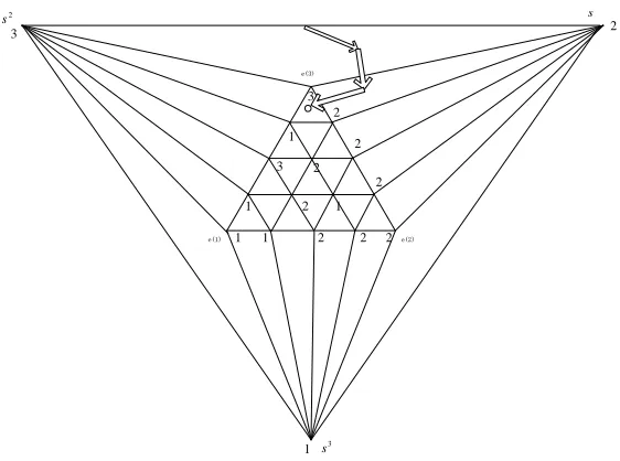
5 Monte Carlo Approximation for Solving Sequential Auctions 67 5.1 Model . . . 68
5.1.1 Sequential Game Representation . . . 70
5.2 Leveraging Substructure in the Complete Information Game . . . 72
5.3 Monte Carlo Approximation . . . 74
5.4 Empirical Results . . . 76
5.5 Convergence of MCA Policies . . . 81
5.6 Related Work . . . 86
5.7 Conclusions . . . 88
6 The Non-Existence of Equilibrium in Sequential Auctions when Bids are Revealed 90 6.1 Introduction . . . 90
6.2 The Model . . . 91
6.3 Symmetric Equilibria in Sequential Auctions . . . 93
6.3.1 Weber’s Equilibrium . . . 93
6.3.2 A Counter Example when Bids are Revealed . . . 93
6.3.3 Non-Existence of Symmetric Equilibrium in Sequential First-Price Auctions 95 6.3.4 Non-Existence of Symmetric Equilibrium in Sequential Vickrey Auctions . 102 6.4 Non-Existence of Asymmetric Equilibrium . . . 111
6.5 Conclusions . . . 113
7 Summary and Future Work 114 7.1 Summary of Contributions . . . 114
Appendices 117
A Mathematics Prerequisites 118
B Notation 120
List of Figures
1.1 An architecture for a flexible decision-making system. . . 6
2.1 The extensive form of Table 2.1. . . 11
2.2 An extensive form game with imperfect recall. . . 12
2.3 A perfect information game. . . 12
2.4 An extensive form game corresponding to the game in Table 2.3. . . 13
2.5 A different extensive form game of Table 2.3. . . 14
2.6 An extensive form game that can be reduced using reduced normal form. . . 16
2.7 Subgame illustration of the game in Figure 2.3. . . 20
2.8 A game of forward induction. . . 22
2.9 Ann-player game illustrating subgame perfect equilibrium. . . 22
2.10 Two extensive games with the same reduced normal form. . . 30
2.11 An extensive game corresponding to the game in Table 2.15. . . 31
2.12 Relationship among different equilibria. . . 33
3.1 Illustration ofK2(m)-triangulation. . . 43
3.2 The Scarf’s triangulation. . . 44
3.3 Illustration of sequence form. . . 46
4.1 Eleven possible equilibrium situations, given thatv1= min i {vi}andv2 = maxi {vi}. 57 5.1 A sequence of two sealed-bid auctions with three agents, one item for sale in each auction, and two bid levels. . . 71
5.2 Our agent’s expected payoff in the {5,4,s-s-s-s} market scenario with the other agents’ valuations drawn from a uniform distribution and equation (5.2) is used to update policies. . . 79
5.3 Our agent’s expected payoff in the {5,4,s-s-s-s} market scenario with the other agents’ valuations drawn from a uniform distribution and equation (5.1) is used to update policies. . . 80
5.5 Our agent’s expected payoff in the {5,4,s-s-s-s} market scenario with the other agents’ valuations drawn from a left-skewed Beta distribution. . . 82 5.6 Our agent’s expected payoff in the{5,5,s-2Mth} scenario with the other agents’
valuations drawn from a uniform distribution. . . 83 5.7 Our agent’s expected payoff in the {5,5,s-2PYB} scenario with the other agents’
valuation are drawn from a uniform distribution. . . 84 5.8 Comparison of our agent’s expected payoff among different types of auctions by
using MCA strategy while the other agents’ valuation are drawn from a uniform distribution. . . 85 5.9 Comparison of the expected social welfare among different auction scenarios when
our agent plays its MCA strategy and the other agents’ valuation are drawn from a uniform distribution. . . 86 5.10 Comparison of the expected revenue among different auction scenarios when our
List of Tables
2.1 A sealed bid auction game. . . 10
2.2 The normal form representation of Figure 2.3. . . 13
2.3 A sealed bid auction game corresponding to the game in Figure 2.4. . . 14
2.4 The multiagent representation form of the game in Figure 2.3. . . 15
2.5 The normal form representation of Figure 2.6. . . 16
2.6 The purely reduced normal form representation of Figure 2.6. . . 16
2.7 The fully reduced normal form representation of Figure 2.6. . . 17
2.8 A game of matching pennies. . . 18
2.9 Battle of the Sexes. . . 19
2.10 A game of prisoner’s dilemma. . . 20
2.11 An incomplete information sealed bid auction. . . 23
2.12 A game in strategic form. . . 27
2.13 A normal form game. . . 28
2.14 A 3-person game. . . 29
2.15 A normal form game corresponding to the game in Figure 2.11. . . 31
2.16 Categories of equilibria. . . 32
3.1 Algorithms to find a single equilibrium. . . 48
3.2 Algorithms to compute all equilibria. . . 49
6.1 The expected utility of bidder0in the sequential FPSB auctions. . . 95
6.2 The expected utility of bidder0in the sequential Vickrey auctions. . . 103
Chapter 1
Introduction
Auctions have permeated into our society more than ever. More and more companies utilize auctions as an important channel in marketing their products. Millions of people purchase commodities from Internet auction sites, such as eBay, Priceline.com, Yahoo Auctions, and Amazon Auctions. As a glimpse of the size of these auction markets, in 2003 the gross revenue of eBay reached 15 billion [34].
What is an auction? An auction is a market institution in which prices and resource allocation are determined by an explicit set of rules on the basis of bids from the market participants [62].
An auction is a dynamic pricing tool that allows sellers and buyers to reach an agreement on prices and allocations. Either sellers or buyers or third parties can initiate an auction. Sellers might want to utilize auctions to sell items at a higher price to some more affordable customers, and hence to increase the overall revenue; while buyers might enjoy a more flexible market when participating in auctions and avoid overpaying. Usually in auctions, the market is efficient when the buyers with the highest valuation win the items.
The research on auctions has burgeoned in the past decades. Many auction mechanisms, especially the standard auctions like the English, the Dutch, the first-price sealed-bid, and the Vick-rey auctions [41], have been discussed in great detail in literature (see, for example [41, 51, 62, 72, 73]). The auction mechanisms discussed in this thesis include:
submits a single bid independently, without observing others’ bids, and the winner with the highest bid pays the price of the highest bid.
• Second-Price Sealed Bid (SPSB or Vickrey) Auction: In the Vickrey auction, each bidder submits a single bid independently, without observing others’ bids, and the winner with the highest bid pays the price of the second highest bid.
• English Auction: In the English auction, the price is successively increased until only one bidder remains, and the winner pays the final price.
• Dutch Auction: In the Dutch auction, the auctioneer starts at a high price, and then lowers the price continuously. The first bidder who calls out wins the object and pays at the current price.
• Mth-Price Auction: There are M objects for sale in an Mth-price auction. In Mth-price auctions, winners pay at the price of the lowest winning bid. The Mth-price is a little bit different from the uniform auction [106], in which winners pay the highest rejected bid or (M + 1)thprice, like in the Vickery auction.
• Pay-Your-Bid Auction: A pay-your-bid auction is a multi-object auction, in which winners
pay the prices they bid. Pay-your-bid auctions are also classified as discriminatory auctions in some literature [106], because winners pay different prices for identical items.
Wurman, et al. present an auction parametrization which is useful for designing auction mechanisms [112]. In their work, the parameterization of the auction design space is broad enough to encompass most of the classic auctions and many others [109]. There are three axes are intro-duced: bidding rules, clearing policy, and information revelation policy. The elements in each axis are listed as following.1
1. Bidding Rules
• Restrictions on sellers; buyers; objects; number of auctions; expressiveness; bid refine-ments; schedule; activity.
2. Clearing Policy
• Clear timing; closing conditions; matching function; tie breaking; auctioneer fees.
1
3. Information Revelation Policy
• Price quotes; quote timing; order book; transaction history.
A sequential auctions is a market scenario that consists of a sequence of individual auc-tions. In both local auction houses and on-line auction sites it is quite common to see identical or nearly-identical items sold in a sequence. Examples include auctions for electronic devices, art, wine, fish, flowers, mineral rights, satellite broadcast licenses, government debts, and many oth-ers [27]. Among those reported in the academic literature are the sequential sale of 120 identical cases of wine in 1990 at Christie’s of Chicago [63] and the sale of pelts on the Seattle Fur Ex-change [52]. eBay, the world’s largest electronic auction, can be viewed as an unending series of auctions for hundreds of thousands of nearly identical items.
The vast number of trading opportunities and the increasingly fluid markets bolsters the need for automated trading support in the form of trading agents—software programs that partici-pate in electronic markets on behalf of a user. Simple bidding tools, like eSnipe2and AuctionBlitz3 enable bidders to automate submission of last-second bids on eBay. However, these tools lack the sophistication that bidders require when faced with a plethora of sequential auctions possibly hosted at multiple auction sites.
The literature on sequential auctions dates back to Vickrey [102], in which he obtains an equilibrium solution for a sequence of first-price auctions with bidders whose single-unit-demand valuations are drawn from a uniform distribution. Since Vickrey’s original work, a great deal of research has been directed towards understanding sequential auctions. Milgrom and Weber [74] discuss the equilibrium solutions and price trends under more general assumptions. The following year, Weber published a sequential auction model [106] that served as a foundation for many of the papers that followed.
The rest of the literature on sequential auctions identifies a wide variety of research areas. Bernhardt and Scoones [5] find that a more dispersed valuation distribution on one item may yield more revenue for the seller. Gale and Stegeman [27] model two completely informed and asymmet-ric buyers bidding forN identical objects fromN sellers sequentially under complete information by assuming that the value of one object depends on the number of objects obtained. Branco [8] models a two-unit sequential English auction when some bidders have superadditive (complemen-tary) values for the objects. Sørensen [97] finds that, in theory, objects are allocated as a bundle
2
http://www.esnipe.com
3
more often than as independently in sequential auctions for complements.
A sequence of prices is a martingale if prices drift neither up nor down over time [106]. Milgrom and Weber [74, 106] predict a martingale among the price trend in symmetric equilibrium of single-unit demand sequential auctions. However, experiments often show the price declines, which is called the declining price anomaly or afternoon effect [63, 85]. Beggs and Graddy [4] report some empirical afternoon effect results from art auctions. Some researches find that the anomaly is explained by varying the assumptions. For example, Engelbrecht-Wiggans finds that prices will on average have a downwards trend in a sequence of auctions for a large enough number of stochastically equivalent objects with bounded values [17]. McAfee and Vincent explain that sequential auctions with risk averse bidders will have a decreasing pattern of prices [63]. Gale and Stegeman [27] claim prices decline weakly along any equilibrium path in a multi-unit demand model with two asymmetric buyers. Katzman [39] concludes that the price trend may decrease in expectation in a game of two second price auctions with multiunit demand, symmetric, incomplete information, when there is a high degree of ex ante asymmetry of bidder beliefs.
Pitchik and Schotter [85] present some laboratory results from an experiment with budget-constrained, perfectly informed bidders. They conclude that bidders attempt to exploit the con-straints of others, and in doing so, bidders might bid up the prices in early stages. As a result, the opponents might deplete their budgets and the later auctions might become less competitive [41, 85].
It is commonly believed that bidders’ behaviors will change when they are forced to pay an entry fee or when there is a reserve price. von der Fehr [103] shows that prices will typically decline for later units in a model with participation constraints, e.g., entry fee. McAfee and Vincent [64] prove revenue equivalence between repeated first price and second price sequential auctions with reserve price.
[20] finds that in two-bidder, multi-unit demand, sequential auctions, an uninformed bidder may have strictly more expected profit than an informed bidder.
Elmaghraby [15] shows that the order in which heterogeneous items are auctioned will influence the outcome. Gale and Hausch [25] show that giving the buyer the right-to-choose her preferred item from the remaining items induces declining prices. Jeitschko [37] models n ≥ 3 single-unit demand bidders in a sequential auction with a stochastic number of identical objects. Gale, Hausch and Stegeman [26] model two identical suppliers in sequential second price auctions with subcontracting. Krishna [50] shows that deterring entry at one stage affects the cost of doing so in later stages in a monopolist model.
Recently, the design of more sophisticated trading agents has attracted the attention of researchers in artificial intelligence and other related fields [9, 30, 90, 100, 108]. In most of these studies, the agents are designed for a particular marketplace and lack flexibility to adapt to other market configurations.
The vast majority of auction research models them as games. An equilibrium strategy is a stable solution in which no player wants to unilaterally deviate from the strategy profile. Thus, finding optimal strategies in auctions is naturally transformed to finding the equilibrium strategies in the auction games.
The literature on sequential auctions provides answers for specific cases but not for gen-eral cases. When the strategy space is discrete and finite, however, the cost of doing the computation increases exponentially in terms of memory and computation time. When the strategy space is con-tinuous or infinite, to date, there are few explicit and generic algorithms for solving this kind of infinite games. A decision-making system in these complex economic settings require not only economic but also computational efficiency.
There are two research gaps to be bridged. First, as more and more auction mechanisms are introduced, it is useful to provide closed-form solutions. Second, urged by the need of industrial application, it is useful to design heuristic algorithms for large-scale problems which have not yet been solved analytically.
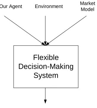
The flexible decision-making system should be designed to generate the optimal strategies for agents automatically, as illustrated in Figure 1.1.4 To make use of the system, we need to specify our agent, the environment, and the market model.
• Our agent: Our agent is described by a utility function, a preference structure, and a
distribu-4
Flexible
Decision-Making
System
Environment
Our Agent Market
Model
Strategies
Figure 1.1: An architecture for a flexible decision-making system.
tion function, etc.
• Environment: The environment might be defined by a set of auction rules.
• Market model: We model other agents explicitly. The system knows about whether the agents
know the strategies of each other and what strategies the other agents use. For example, some agents may use equilibrium strategies while the others use myopic strategies. A market model also includes whether the other agent’s preferences and other information are known [110].
This thesis aims to provide answers to several issues. On the theory side, I provide closed-form solutions to FPSB auctions and sequential FPSB auctions. I also analyze the non-existence of equilibrium in two sequential auction models. On the algorithm side, I present a heuristic algo-rithm as part of a flexible decision-making system to compute solutions for sequential auctions with discrete bids [10].
In Chapter 2, I review some basic concepts of game theory and provide a brief survey on Nash equilibrium and its refinements. Chapter 3 provides a review of the state-of-art algorithms for computing equilibria.
with discrete bids under both complete information and incomplete information.
Chapter 5 focuses on a flexible decision-making system for sequential auctions with dis-crete bids. I present a heuristic approach using Monte-Carlo approximation. This system enables users to compute solutions for different sequential auction models more efficiently than existing algorithms.
In Chapter 6, I study the impact of information in sequential auctions when altering dif-ferent information revelation policies. I prove the non-existence of pure-strategy symmetric equilib-rium in both symmetric sequential first-price sealed-bid auctions and symmetric sequential Vickrey auctions.
Chapter 2
Strategic Equilibria
In a broad sense, a game may refer to any social situation involving two or more individu-als [78].1 Individuals are also called players, agents, or decision-makers. Each individual is usually assumed to be rational, which implies that every player always maximizes his utility [28]. Game theory is the study of the noncooperation and cooperation between these rational players.
An equilibrium is defined as a state of a system that the system tends to move back to the same state when the system is perturbed from its original state. Equilibrium in a game is also called
strategic equilibrium. Finding strategic equilibrium in games is a major task of game theorists.
2.1
Basic Concepts
For the sake of completeness, a brief review of the relevant definitions is provided.
An eventE is common knowledge if all players know thatE occurred, and all players know that all players know thatEoccurred, and so on, ad infinitum.
A game is of certainty if there is no stochastic events, which are typically characterized as a move by nature. If there is a move by nature, the game is said to have uncertainty.
A game is one of symmetric information if an agent’s information state has the same ele-ments as those of every other agent. Otherwise the game is said to be one of asymmetric information.
1
A game is one of incomplete information if some or all of players lack full information about the timing of the game, the set of strategies, or the payoffs of players [28]. For example, nature moves first and is unobserved by at least one of the agents. Otherwise, the game is one of
complete information.
A game is one of perfect information if each agent knows every action of the agents that moved before him at every point. Otherwise, it is one of imperfect information.
A strategic form game is finite if the number of players and the number of strategies is finite.
There are two kinds of games that have complete information but imperfect information. In the first scenario, the agents move simultaneously. In the second scenario, nature moves without revealing information immediately to all agents.
2.2
Game Models
A game model is a description of a game. Game models are also called game forms. Different forms abstract the game from a different perspective. To find a solution for a game, one builds a model of the game and then solves for an equilibrium of the model [23]. Due to variations in game models and copious equilibrium concepts, it is possible that we might have different answers as well as different specific solution procedures to the same game.
The two most important game forms are the extensive form and the normal (or strategic) form. In addition to these two forms, there are also the agent normal form and the reduced normal form. Due to limited space, we discuss only these four game models.2
2.2.1 Strategic Form and the Normal Representation
A strategic form has three elements: a set of players,A, a set of possible (pure) strategies,{Si}i∈A,
and a set of utility (payoff) functions, {ui}i∈A. Thus, a strategic form gameΓcan be denoted by
Γ ={A,{Si}i∈A,{ui}i∈A}.
We letσdenote a strategy profile of the game. Letσibe a strategy profile of playeriand σi,s be the choice probability of each pure strategy,s, in playeri’s strategy set,Si. Ifσi,s∈ {0,1},
we callσ a pure strategy profile. Otherwise,σ is a mixed strategy profile. For example, in a
two-2
Bidder 2 (v=2)
1 2
Bidder 1 1 0.75, 0.5 0,0 (v=2.5) 2 0.5, 0 0.25, 0
Table 2.1: A sealed bid auction game.
player game, each player has two actions,{a, b}. For a pure strategy profile in which Player 1 uses actionband Player 2 uses actiona, the profile is written asσ ={b, a}. For a mixed strategy profile in which Player 1 has1/2probability to use actionaand Player 2 has1/3probability to use action
a, we haveσ ={(1/2,1/2),(1/3,2/3)}.
As an example, a strategic form of a sealed bid auction, with two players and two bid values for each player, can be expressed as in Table 2.1, which is the normal representation of the game. In strategic forms, game theorists assume that players choose their strategies independently [80]. So, all the strategies in strategic form can be expressed in independent vectors. As a result, a strategic form game is equivalent to a normal form game.
2.2.2 Extensive Form
The extensive form is more richly structured than the normal form. Normally, we use a tree graph to depict an extensive form game. The tree consists of a set of branches, each of which connects two nodes. The first node is called root, which represents the beginning of the game and the bottom nodes are called terminal nodes and represent the end of the tree.
An extensive form game,Γe, includes six elements in which the first three elements are
almost the same as in a strategic form game [23, 114]. 1. A set of players,A, each of which has a player label.
2. The strategy spaceSi(ξ)of each player,i, at each information state (also called information
Figure 2.1: The extensive form of Table 2.1.
3. The players’ payoff functions,{ui}i∈A. Normally, we label the payoff values at the terminal
nodes.
4. The order of moves, i.e., who moves when.
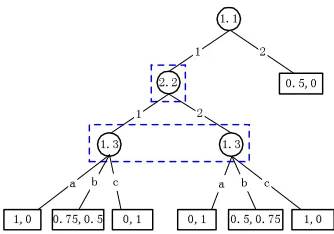
5. The information state,ξ, of each player when she will move. We denote the set of information states asΞ.
6. The stochastic events, which are encoded chance nodes annotated with their probabilities. An example is shown in Figure 2.1. The first “1” in “1.1” identifies Player 1, where the second “1” identifies the first information state of Player 1. There are two “2.2”’s in the game which indicates that there is only one information state for Player 2 because Player 2 cannot observe Player 1’s action. The single “1” and “2” along the branches are the feasible actions a player has in the information state.
A behavioral strategy profile in extensive forms refers to a probability over the set of possible strategies for each possible information state of each player. A behavioral strategy profile is very similar to a strategy profile defined in the normal form. The difference is that a behavioral strategy profile is related with information states. Let σ denote a behavioral strategy profile. Let
σξ,i be a behavioral strategy profile of player i at information state ξ, and σξ,i,s be the choice
probability of each pure strategy, s, in playeri’s strategy set,Si(ξ), at information state ξ. Thus,
we haveσ = {σξ,i}i∈A = {σξ,i,s}s∈Si(ξ),i∈A. Ifσξ,i,sequals 0or1, we callσ a pure behavioral
strategy profile. Otherwise, σ is a mixed behavioral strategy profile. For example, in Figure 2.2,
0.5,0
2.3
c d
0.75,0.5 0,0
1.1
2 1
2.2
b a
2.3
c d
0,0 0.25,0.75
Figure 2.2: An extensive form game with imperfect recall.
Figure 2.3: A perfect information game.
Bidder 2
1,1 1,2 2,1 2,2
Bidder 1 1 0.75, 0.5 0.75, 0.5 0,0 0,0 2 0.5, 0 0.25, 0 0.5, 0 0.25, 0
Table 2.2: The normal form representation of Figure 2.3.
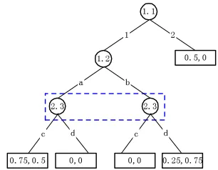
Figure 2.4: An extensive form game corresponding to the game in Table 2.3.
The Strategic Form Representation of Extensive Form Games
The normal form and extensive form are the two most common models for games. Even with these two models, we might have different results when we solve the same game.3
An extensive form can give us more information than a normal form game. It is possible to convert an extensive form game to strategic form, but we may lose information about the sequence of moves. To express this in normal form, we will assume that a player makes a complete contingent plan in advance [23]. Let those strategies inΓebe the pure strategies inΓand let payoff functions
be the same. Thus, the strategic form of the game in Figure 2.1 can be represented as in Table 2.1. In Figure 2.3, Player 2 has two information states corresponding to different moves by player 1. Totally, there are four pure strategy profiles,{1,1},{1,2},{2,1},{2,2}, if represented in normal form. As a result, the normal form of the extensive form game in Figure 2.3 can be expressed as in Table 2.2.
It is not surprising that a normal form might have multiple extensive form representations. Consider Figure 2.4. The normal form representation of this game is shown in Table 2.3, which is very similar to Table 2.1. The only difference lies in that the payoff functions are the same when
3
Bidder 2
1 2
Bidder 1 1 0.75, 0.5 0,0 2 0.5, 0 0.5, 0
Table 2.3: A sealed bid auction game corresponding to the game in Figure 2.4.
Figure 2.5: A different extensive form game of Table 2.3.
Player 1 chose “1” in both tables. Now, let us define an extensive form representing from the normal form game as shown in Table 2.3. From the same normal form game, we may have two different extensive form games, which are illustrated in Figure 2.4 and Figure 2.5. This interesting phenomenon confirms that we might lose some information when a normal form is represented from an extensive form.
Agent Normal Form
Defined by Selten [94], the agent-normal form representation is a modification of the extensive form, in which each information state in an extensive form game is associated with a different “temporary” agent. Those temporary agents share the same payoffs with the original agent. Some literature [23] also calls agent-normal form the agent strategic form or multiagent representation
form. Similar to the relation of the normal form to the extensive form, a multiagent representation
Bidder 2
1 2
Bidder 3 Bidder 3
1 2 1 2
Bidder 1 1 0.75,0.75,0.5 0.75,0.75,0.5 0,0,0 0,0,0 2 0.5,0.5,0 0.25,0.25,0 0.5,0.5,0 0.25,0.25,0
Table 2.4: The multiagent representation form of the game in Figure 2.3.
Table 2.2 isA={1,2}; the strategy profiles areS1 ={1,2}andS2 ={(1,1),(1,2),(2,1),(2,2)};
and the payoff functions are shown in Table 2.2. In comparison, the set of players in Table 2.4 is
A={1,2,3}; the strategy profiles areS1 ={1,2},S2 ={1,2}, andS3 ={1,2}; and the payoff
functions are shown in the Table 2.4. These two representations may result in different solutions as shown in a later discussion on perfect equilibrium, in the sense that the multiagent representation form is to rule out correlation between the “mistakes” of the same player in different stages of the game [94].
Reduced Normal Form
A reduced normal form,G, is a strategic form in which all pure strategies of a player that are convex combinations of other pure strategies of the same player have been deleted [43]. Let us examine some prerequisite concepts.
Definition 2.2.1. Given any two strategies,cianddi, in the strategy setSiof playeri,cianddiare said to be payoff equivalent if and only if for alls−i ∈S−iandj∈A
uj(s−i, ci) =uj(s−i, di).
!"
# $
" " %
!" &!
' '
# $
" "
%
&!" !
Figure 2.6: An extensive form game that can be reduced using reduced normal form.
Bidder 2
1 2
1a 1,0 0,1
1b 0.75,0.5 0.5,0.75
Bidder 1 1c 0,1 1,0
2a 0.5, 0 0.5, 0 2b 0.5, 0 0.5, 0 2c 0.5, 0 0.5, 0
Table 2.5: The normal form representation of Figure 2.6.
Bidder 2
1 2
1a 1,0 0,1
1b 0.75,0.5 0.5,0.75
Bidder 1 1c 0,1 1,0
2. 0.5, 0 0.5, 0
Bidder 2
1 2
1a 1,0 0,1
Bidder 1 1c 0,1 1,0 2. 0.5, 0 0.5, 0
Table 2.7: The fully reduced normal form representation of Figure 2.6.
Definition 2.2.2. A strategyeiinSiis randomly redundant if and only if it is a convex combination of the other pure strategies, where there is a probability distribution σi in ∆(Si), the set of all
randomized strategies for Playeri, such thatσi(ei) = 0and for alls−i∈S−iandj∈A
uj(s−i, ei) =
X
di∈Si
σi(di)uj(s−i, di).
For example, the strategy1bis redundant because its payoff function can be expressed by a convex combination of strategies 1a and 1c. A purely reduced normal representation is a fully reduced normal representation if it deletes all the randomly redundant strategies. The fully reduced normal representation of Figure 2.6 is shown in Table 2.7. Unless specified otherwise, we regard the reduced normal representation as the fully reduced normal representation.
2.3
Equilibrium Concepts
A static (simultaneous) game is one in which players will move simultaneously, without knowledge of the strategies that are being chosen by other players. A static game can be easily modeled as a normal form game.
A dynamic game will specify the order of moves. Unlike static games, players have at least some information about the choices made on past moves. The extensive form is usually used to express a dynamic game.
Player 2 Head Tail Player 1 Head 1,-1 -1,1 Tail -1,1 1,-1
Table 2.8: A game of matching pennies.
The second milestone was the introduction of subgame perfect equilibrium for dynamic games with complete information. Selten [94] refines the concept of Nash Equilibrium to subgame perfect equilibrium which can be applied to dynamic games and is computed using backward induction. The third milestone is Harsanyi’s Bayesian equilibrium [31] which enables the agents in incomplete information games to choose strategies conditionally based on the perceptions of what the other agents are likely to do.
We discuss these three milestone equilibria together with other important equilibria in the following.
2.3.1 Nash Equilibrium
A Nash equilibrium describes a state of a multi-agent system in which no one can benefit by uni-laterally changing her strategy. For example, in the game of Figure 2.1, the strategy profiles{1,1} and{2,2}are Nash equilibria.
We may explain the Nash equilibrium in another way. Suppose there is one agreement that all players promised to comply with prior to the game. This agreement is self-enforcing (or strategically stable) if no one would prefer to deviate and choose some strategy other than that specified in the agreement. Thus, to be self-enforcing, it is necessary that the agreement form a Nash equilibrium [49].
It is worth noting that, at the beginning of game theory, “more attention was focused on the cooperative analysis that von Neumann favored” [80]. Together with von Neumann’s “cooperative” game theory, Nash equilibrium provides a “complete general methodology” to analyze all games [80]. In fact, a cooperative game can be reduced to a non-cooperative games in which “the steps of negotiation become moves” in the non-cooperative game [83]. Thus, Nash equilibrium applies to both cooperative games and non-cooperative games.
Female Badminton Movie
Male Badminton 2,1 0,0
Movie 0,0 1,2
Table 2.9: Battle of the Sexes.
[83]. However, not every game has pure strategy Nash equilibrium; some games may have only mixed strategy equilibria. A classic example is “matching Pennies”, shown in Table 2.8. In this game, two players simultaneously announce heads or tails. If the announcement matches, Player 1 wins; otherwise, Player 2 wins. There is no pure strategy Nash equilibrium in this game. The only stable situation is that both players play randomly between their two possible pure strategies with probabilities(1/2,1/2).
A game may have more than one Nash equilibrium. This problem often makes it hard to predict which Nash equilibrium will be played, and may complicate the computation of Nash equilibrium. We call this problem multiplicity. To solve this problem, game theorists try to provide some basis for claiming one equilibrium is better than another.
An allocation is Pareto efficient if no agent can be better off without making the others worse off. One criterion to find “better” equilibria is to look for Pareto efficient outcomes within the set of Nash equilibrium. If there are any overlaps, we call these overlapping Nash equilibria Pareto
dominant. For example, in the game of Figure 2.1, the strategy profile{1,1} is Pareto dominant {2,2}, and we can argue that it is a better equilibrium. However, this variant is often not conclusive.
Focal-point Effect The Focal-point effect argues that some of the given multiple Nash equilibria will be more plausible due to special properties they have. For example, suppose there are two Nash equilibria in one game, one pure strategy and another one mixed strategy. Some theorists argue that it is more preferable for the players to play the pure strategy [78]. Another focal-point effect example is Battle of the Sexes shown in Table 2.9. {Badminton, Badminton} and{M ovie, M ovie}are two Nash equilibria. However, suppose the female has some priority in the relationship; both players may be able to determine that {M ovie, M ovie} will likely be the final result.
dom-prisoner 2 Testify Conceal prisoner 1 Testify -3,-3 0,-5
Conceal -5,0 -1,-1
Table 2.10: A game of prisoner’s dilemma.
()(
* ( *)*
( *
+),-.+)- +.+
*)*
( *
+),-.+)- +.+ *)/
( *
+)*-.+ +)-.+
*)/
( *
+)*-.+ +)-.+
012 3456789 7 0:2 3456789 5 0;2 3456789 <
Figure 2.7: Subgame illustration of the game in Figure 2.3.
inant strategies is called a dominant equilibrium. A dominant equilibrium is a Nash equilibrium. A famous example is the Prisoner’s Dilemma game. As shown in Table 2.10, if both prisoners do not testify, they each get −1 rewards; if both testify, they each get −3 rewards. If one tes-tifies and the other does not, the former one gets 0 reward while the latter one gets −5. In the Prisoner’s Dilemma, each player has a dominant strategy. However, the resulting equilibrium is Pareto dominated by an alternate outcome in which each player chooses the dominated strategy. It turns out that {testif y, testif y} is the dominant strategy. It is worth noting that there is no Pareto dominance among equilibria in this game because there is only one Nash equilibrium. In fact,{testif y, testif y}is the only solution which is not Pareto efficient.
2.3.2 Subgame Perfect Equilibrium
A subgame is a component of a game. Letxbe a node of an extensive form game, Γe. Letg(x)
be the set of all nodes and branches that follow x, including the node x itself. The node x is a
subroot if, given any other node,x′, inΓe, which happens at the same time atxor thereafter, either
g(x′)∩g(x) = ∅org(x′) ⊆ g(x). We refer to g(x) as a subgame, γe
x, of Γe. Γeis a subgame
itself. For example, the game in Figure 2.3 has three subgame, as shown in Figure 2.7. In another example shown in Figure 2.1, the only subgame is the game itself. Because the information state of Player 2 cannot be separated, and the closest root of both nodes of this information state is the root of information state 1.
A behavioral strategy profile is a subgame perfect equilibrium if it introduces a Nash equi-librium to every subgame [94]. If there is more than one subgame inΓe, we may find an equilibrium path, in which, the restriction of the behavioral strategies to each subgame is an equilibrium. Let
us look at the game in Figure 2.7 again. The Nash equilibrium of subgamebis{1}. In subgamec, either{1} or{2}could be the equilibrium solution for Player 2. Regardless of which one Player 2 picks, or whether she chooses a convex combination in subgamec, Player 1 will choose strategy {1} in subgamea. Thus, there is only one subgame perfect equilibrium in this game, rather than two Nash equilibria as shown in Figure 2.3.
The concept of subgame perfect equilibrium is stronger than Nash equilibrium. If there is only one subgame inΓe, each subgame perfect equilibrium is a Nash equilibrium, and vice versa.
However, if there is more than one subgame in Γe, the set of Nash equilibrium is a superset of
subgame perfect equilibrium while every subgame perfect equilibrium is a Nash equilibrium.
=>?@=
A>B
C D
=>E?@=>? =@=
F>F
A F
F>A
G H
A>B
C D
=@= =>A?@=>E?
Figure 2.8: A game of forward induction.
III J
I
J K
L
M I
M
NOPQQQPOR L STUVWXXXWTUVY
K Z[\]Z[\ K
L
^ I
^
L NO_`PQQQPO_`R
K NaPQQQPaR
Figure 2.9: Ann-player game illustrating subgame perfect equilibrium.
to happen in the subgame. As a result, Player 2 should choosecin the subgame, so{1, a, c}is the only equilibrium in the forward induction.4 Thus, forward induction may provide different solutions from backward induction. See page 192 in [78] for more examples.
Backward induction is not the only problem in subgame perfect equilibrium. Like Nash equilibrium, subgame perfect equilibrium assumes that all players are perfectly rational. Thus, all players expect an equilibrium in the whole game and the same equilibrium in every subgame. That is to say, subgame perfect equilibrium does not allow for imperfect play in the game. Consider the game in Figure 2.9. {b, b, ..., b}is the only subgame perfect equilibrium and only forward induction equilibrium. However, there is one credible threat to{b, b, ..., b}. To show why, suppose that the first player has probability of(1−P)to choosea. If all players have the same probability to do so, the overall probability that all players will playbisPn. Ifnis large,Pnwill be small. So, in this sense,
{b, b, ..., b} will not be a good solution. As a re-examination of his subgame perfect equilibrium
4
Bidder 2
Low Valuation High Valuation
c d c d
Bidder 1 a 0.75, 0.5 0,0 0.75, 1 0, 1 b 0.5, 0 0.25, 0 0.5, 0 0.25, 0.5
Table 2.11: An incomplete information sealed bid auction.
concept, Selten [94] introduces a small “mistake” for every possible move of all players. We will touch this concept in sequential equilibrium and (trembling hand) perfect equilibrium.
2.3.3 Bayesian Equilibrium
Nash equilibrium assumes complete information. Difficulties arise in games of incomplete infor-mation in which players do not know each other’s characteristics and hence the payment functions are no longer common knowledge. We illustrate this problem by discussing a two-person sealed bid auction, illustrated in Table 2.11. In this game, if bidder 2 has a low valuation of one item, {low, low} is a weakly dominant Nash equilibrium. However, if bidder 2 has a high valuation, {high, high}is a weakly dominant Nash equilibrium. So, whether bidder 1 chooses low or high will depend on whether bidder 2 has low valuation or high valuation.
Harsanyi [31] demonstrates that an incomplete information game can be transformed into a game with imperfect information. This kind of transformation is called Harsanyi transformation, in which an incomplete information game is replaced by a game where nature moves first (and chooses the players’ types). As a result, we may have many complete information games with probabilities in accordance with the types of the players.
LetTi be a set of possible types of player i, andT−i denote all possible combinations
of types for the players other than i. Let ti be a typical type in Ti, and let t−i be any possible
combination of types for the players other than i. Let pi be a probability function from Ti to
∆(T−i), which is the set of probability distributions overT−i. We definepi(t−i|ti)for playerias
the probability that the other players havet−iwhile playeriis inti. uidenotes the utility function
of playeri. We define a Bayesian game as a profile,
Γb ={A,{Si}i∈A,{Ti}i∈A,{pi}i∈A,{ui}i∈A}.
player is a best response conditional on expectations of others’ best responses, and no one wants to move unilaterally.5 Letσ∗
i(.|tj) denote the best response strategy profile of playerigiventj. We
have
σi∗(.|ti)∈arg max si∈Si
X
t−i∈T−i
pi(t−i|ti)ui(si(ti), s−i(t−i)),(ti, t−i)).
To see how to calculate a Bayesian equilibrium, let us consider the example in Table 2.11. In this game, player 1 has incomplete information while Player 2 has complete information. If Player 2 has a low valuation, Player 2 will playcbecausecis a weakly dominant strategy; otherwise, she will playd. We have
σ1∗(.|t2 =low) =a, σ1∗(.|t2 =high) =b,
σ∗2(.|t2 =low) =c, σ2∗(.|t2 =high) =d.
Suppose that the probability of Player 2’s valuation being low isp. So, for Player 1, the expected payoff if she playsais0.75p. If she playsb, the expected payoff is0.5p+0.25(1−p) = 0.25p+0.25. The critical value ofpisp= 0.5. That is to say, if the probability of Player 2’s valuation being low is less than0.5, Player 1 will playb. For more examples, refer to page 215 in [23].
2.3.4 Perfect Bayesian Equilibrium
In Bayesian equilibrium, each player has a subjective probability distribution over the possible types of the other players. We refer to these subjective probability distributions as prior beliefs. The players do not modify the prior beliefs in the process of the game. However, in multi-stage games, players have the opportunity to observe the outcome of previous stages, and it is reasonable to think that players will modify their prior beliefs in accordance with the new information. The updated belief is called the posterior belief.
Perfect Bayesian equilibrium is an extension of subgame perfect equilibrium to incom-plete information games. To formally define perfect Bayesian equilibrium, we letaξi be the action of playeriat an information stateξ.6 Letpei(t−i|aξ−i)be the posterior probability oft−igiven that
5
A Bayesian equilibrium is also called a Bayes-Nash equilibrium, or expectation equilibrium.
6
playeriobserves the other players’ moves leading to the information stateξ. A behavioral strategy profile is a perfect Bayesian equilibrium if at each information stateξ, we have
1. A player’s strategy conditional ontiis a best response to the other players’ best response. For
alli∈Aandξ∈Ξ, we have
σξ,i∗ (.|ti)∈arg max si∈Si(ξ)
X
t−i∈T−i e
pi(t−i|aξi)ui(si, s−i, ti).
2. pei(t−i|aξ−i)is updated froma ξ
i ands−iusing Bayes’ rule whenever possible.
Thus, a perfect Bayesian equilibrium is a set of behavioral strategies and beliefs such that strategies are optimal given the beliefs at any stage of the game. The beliefs are updated from prior beliefs, equilibrium strategies, and observed actions using Bayes’ rule.
2.3.5 Sequential Equilibrium
In perfect Bayesian equilibrium, there is no explicit definition of posterior probability when the observation probability is zero. As a result, there is no explicit definition of those strategies off the equilibrium path [114]. In this sense, perfect Bayesian equilibrium cannot guarantee an equilibrium solution for every subgame. Selten [94] introduces a concept referred to as “trembling hand per-fection” to capture the notion that players may make errors with small probabilities. The trembling hand is a vivid description of “slight mistake” in which a player will do something wrong because she cannot hold her hand firmly. By introducing trembling, we enable the game to reach every information state.
This concept is applied in both (trembling hand) perfect equilibrium and sequential
equi-librium. We introduce sequential equilibrium at first, because sequential equilibrium is simpler and
normally easier to compute.
Kreps and Wilson [48] define (σ,µ) as an assessment, whereσ is a behavioral strategy profile andµis a set of beliefs at all information states. LetΣbe the set of allσs. σi(ξ)denotes the
strategy profile of playeriat information stateξandσ−i(ξ)denotes the strategy profile of all players
exceptiat information stateξ. ui(ξ)denotes the utility of playeriatξ. Letµi(ξ)be the posterior
1. (σ,µ) is sequential rational, that is, for every information stateξ,
ui(ξ)(σ|ξ, µ(ξ))≥ui(ξ)((σ
′
i(ξ), σ−i(ξ))|ξ, µ(ξ)),
for alli∈A,ξ∈Ξandσ′ ∈Σ.
2. (σ,µ) is consistent if there exists a sequence of strictly mixed (behavioral) strategy(ˆσk)∞
k=1,
and associated beliefs(µk)∞
k=1determined by Bayes’ rule, such that
(σ, µ) = lim
k→∞(ˆσ
k, µk).
There are two points worth noting. First, players will adhere to the equilibrium profileσat any information state including those off the equilibrium path. This is the same as subgame perfect equilibrium. Secondly, the behavioral strategies σ can be pure strategies, where(σ, µ) are limits of mixed strategies and associated beliefs. For example, consider a simple game in which Player 1 has a two-action strategy space. Suppose that σ1 = (1,0) is the only pure strategy sequential
equilibrium for Player 1. As required by the trembling hand property, we letσˆk
1 = (1−ǫk, ǫk).
Whenk→ ∞, we haveǫk →0and(ˆσ1k, µk)→(σ1, µ).
2.3.6 Perfect Equilibrium
First, let us discuss perfect equilibrium in strategic forms. We follow the definition on page 216 in [78]. LetΓ = (A,(Si)i∈A,(ui)i∈A)denote any finite game in strategic form. Let∆(Si)denote the
set of all probability distributions onSiand∆0(Si)denote the set of all probability distributions on Si that assign positive probability to every element inSi. A strategy profileσ in×i∈A∆(Si)is a perfect equilibrium ofΓif and only if there exists a sequence(ˆσk)∞
k=1such that
1. σˆk∈×
i∈A∆0(Si),
2. σi ∈arg max si∈∆(Si)
ui(ˆσ−ki, si), and
3. lim
k→∞σˆ
k
i(si) =σi(si), for alli∈Aand for allsi∈Si.
The first condition requiresσˆkbe a strictly mixed strategy profile in that every pure
strat-egy of every player should have strictly positive probability. This is the same to the requirement in sequential equilibrium. The second condition asserts thatσiis a best response strategy profile given
everyσˆk
Player 2
c d
a 0,1 0,1
Player 1 bx -1,2 1, 0 by -1,2 2,3
Table 2.12: A game in strategic form.
ˆ
σk, is a Nash equilibrium. The third condition tells us that a perfect equilibrium is the converging
limit of a sequence of Nash equilibria. This is a little bit different from sequential equilibrium, which puts more credit on posterior probability so that we may tell which beliefs are “plausible” [23].
However, for the purpose of perfectness, the strategic form is not an adequate represen-tation of the extensive form [94]. In fact, a perfect equilibrium in strategic form may not even be a subgame perfect equilibrium due to “difficulties which may arise with respect to unreached parts of the game ”[94]. To see why, let us look at the example in Table 2.12. In this game,{by, d}is the only subgame perfect equilibrium. It is easy to understand that{by, d} is also a perfect equi-librium. However, {a, c} is also a perfect equilibrium. Suppose Player 1 will play a and, with some small probability, ǫ, tremble tobx and by, Player 2’s expected payoff is 1 + 2ǫif Player 1 plays cand is1 +ǫif she plays d. Since1 + 2ǫ > 1 +ǫ, {a, c} is a perfect equilibrium. Some argue that the mistakes happened in different stages of subgame may be correlated [114]. To re-move such “difficulties”, Selten introduce “agent normal form as a more adequate representation of games with perfect recall” [94], which requires that an agent behaves independently in different stages such that an agent in a different stage looks like a different agent. Selten showed that every perfect equilibrium is always subgame perfect in agent normal form games, but the reverse may not hold.
2.3.7 Proper Equilibrium in Strategic Form
Player 2
c d
ax 5,5 5,5 Player 1 ay 5,5 5,5 bx 7,7 4,0 by 0,0 3,3
Table 2.13: A normal form game.
defines thatσis anǫ-proper equilibrium if and only if 1. σ∈
×
i∈A∆(Si),2. For allci, ei ∈Si,
ifµi(σ−i,[ci])< µi(σ−i,[ei]),thenσi(ci)≤ǫσi(ei).
A randomized-strategy profileσ in
×
i∈A∆(Si)is a proper equilibrium ofΓif and onlyif there exists a sequence(ǫ(k), σk)∞
k=1 such that
1. For allk,σkis anǫ-proper equilibrium,
2. lim
k→∞ǫ(k) = 0, for allk∈ {1,2,3, ...}, and
3. lim
k→∞σ
k
i(si) =σi(si), for allk∈ {1,2,3, ...}, for alli∈Aand for allsi∈Si.
As proved by Myerson [77], every proper equilibrium is a perfect equilibrium, but not vice versa. Consider the game in Table 2.13, the strategy profile
{(1−7ǫ)[ax] +ǫ[ay] +ǫ[bx] + 5ǫ[by],(1−ǫ)[c] +ǫ[d]}
is anǫ-perfect equilibrium. So,{ax, d}isǫ-perfect, as long as0< ǫ < 1/3. However,{ax, d}is not anǫ-proper equilibrium. The reason is thatbyis a worse mistake thanbx for Player 1 because 0ǫ+ 3(1−ǫ)<6ǫ+ 4(1−ǫ). Theǫ-properness condition requires thatσ1(by)/σ1(bx)must be no
more thanǫ[78]. As a fact of matter,{bx, c}is the unique proper equilibrium in this game as long asǫ <2/3. This can be justified by the form
Player 2
c d
Bidder 3 Player 3
e f e f
Player 1 a 0,0,0 0,0,2 0,2,0 2,0,0 b 0,2,0 2,0,2 2,0,2 0,2,0
Table 2.14: A 3-person game.
2.3.8 Persistent Equilibrium in Strategic Form
In the definitions of perfect equilibrium and proper equilibrium, trembles are forced when some of the pure strategies have zero probability. Thus, given that no pure strategy has zero probability, a Nash equilibrium is always perfect and proper [38]. However, this kind of strategy combina-tion, referred to as an inner combinacombina-tion, is not always immune against trembles, and thus could be unstable. Recall the “battle of the sexes” game in Table 2.9. {Badminton, Badminton}, {M ovie, M ovie}, and{(1/2Badminton+ 1/2M ovie),(1/2Badminton+ 1/2M ovie)}are the only three Nash equilibria, which are also perfect and proper. However, {(1/2Badminton + 1/2M ovie),(1/2Badminton+1/2M ovie)}does not have neighborhood stability since any trem-bles, like{((1/2 +ǫ)Badminton+ (1/2−ǫ)M ovie),(1/2 +ǫ)Badminton+ (1/2−ǫ)M ovie)} will cause it to shift to{Badminton, Badminton}.
Here are some prerequisite definitions. A retract of the gameΓis defined as a subsetRof
SifR=
×
i∈A∆(Ri), with eachRibeing a non-empty closed convex subset ofδ(Si). A retractRis absorbingSˆ ifBR(σ)∩R6= 0given thatSˆ is a set of mixed strategiesSˆ ⊆Sand everyσ ∈Sˆ. That is, for every playerithere is aτi∈Risuch thatτiis a best response of playeritoσ ∈R[38].
A retract R is persistent if it is a minimal absorbing retract. A strategy profile σ is a persistent equilibrium ifσis a Nash equilibrium and is a persistent retract [38].
Kalai and Samet prove that any finite game in strategic form has a persistent equilibrium which is perfect and proper. However, there may exist some persistent strategies which are not proper [38]. Let us look at an example, as shown in Table 2.14. In this game, every strategy profile is persistent. However, the strategy{a, c, e}is not perfect.7
7
Game A Game B
1.1
b c def
g h
def
g h
1.2
c 0.5,0.5
1.1
b a
2.2
e f
2.2
e f c 0.5,0.5
0.75,0.75 0.25,0 0,0 0.25,0.25
0.75,0.75 0.25,0 0,0 0.25,0.25
Figure 2.10: Two extensive games with the same reduced normal form.
2.3.9 Stable Equilibrium
As we know, a game in normal form could have different equilibrium solutions, when compared to those in extensive form. Consider the two games in Figure 2.10.8 The reduced normal form game of these two games are the same; however, {c, f} and {a, e} are the perfect equilibria of Game A, while{a, e} is the unique perfect equilibrium of game B. At the same time, backwards induction of the extensive form and the iterated dominance of the normal form do not give us the same “strategically stable equilibrium” [43]. Consider Game B in Figure 2.10 again. Strategybof player 1 is strongly dominated by strategyc. So,{a, e}should be the only equilibrium in iterated elimination of dominated strategies.
Stable equilibrium is a concept developed by Kohlberg and Mertens [43] to solve the above discrepancies. A reduced normal form,G, is where all pure strategies that are convex com-binations of other pure strategies have been deleted [43]. Kohlberg and Mertens point out that a strategically stable equilibrium should depend only on the reduced normal form of the game. A strategically stable set of equilibria ofGmust contain a strategically stable set of equilibria of any
G′, which is obtained fromGby a deletion of any dominated strategy [43].
We defineS as a closed set of Nash equilibrium of G, if for any ǫ > 0 there exists some0 < δ0 ≤ 1, such that the perturbed game, where every strategysof playeriis replaced by
(1−δi)s+δiσi, has an equilibriumǫ-close toS, for any completely mixed strategy vectorσ1, ..., σn
(nplayers) and for anyδ1, ..., δn, (0< δi < δ0). A set of equilibria is stable in a gameGif it is the
minimal set ofS[43].
8
iji
k l mjn
o p
mjn
o p ijm
q r
jst r
js
itui uiti uiti itui
Figure 2.11: An extensive game corresponding to the game in Table 2.15.
Player 2
e f
a 1,-1 -1,1 Player 1 b -1,1 1,-1
c 0.5 0.5
Table 2.15: A normal form game corresponding to the game in Figure 2.11.
Kohlberg and Mertens prove that, in iterated dominance, a stable equilibrium contains a stable set of any game obtained by eliminating dominated strategies. In forward induction, a stable equilibrium contains a stable set of any game obtained by a deletion of any strategy which is an inferior response to the equilibria of the set [43]. However, stable sets might not satisfy the backwards induction requirement. Consider the game in Table 2.15. There are two stable equilibria,{c,(1/4,3/4)}and{c,(3/4,1/4)}. However, in the corresponding extensive form game in Figure 2.11, the only sequential equilibrium is{c,(1/2,1/2)}. The cause of this problem might be because stable equilibrium uses a different game form other than normal form or extensive form representations. Similarly, it may not be a subset of proper or perfect equilibrium.
2.4
Summary
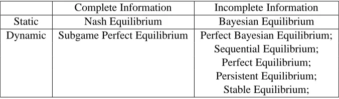
Using static and dynamic as one axis, and information as another, we classify these well-known equilibrium concepts in Table 2.16.
mod-Complete Information Incomplete Information
Static Nash Equilibrium Bayesian Equilibrium
Dynamic Subgame Perfect Equilibrium Perfect Bayesian Equilibrium; Sequential Equilibrium;
Perfect Equilibrium; Persistent Equilibrium;
Stable Equilibrium;
Table 2.16: Categories of equilibria.
els. Usually, Nash equilibrium, proper equilibrium, and persistent equilibrium are solved in normal form. Subgame perfect equilibrium and sequential equilibrium are applied to extensive form games. Perfect equilibrium is discussed in agent normal form. And stable equilibrium is solved in reduced normal form. The choice of a game model to a specific application should depend on the needs of the scenario.
vwx yz {| } ~ } }| | w z {| } ~ } }| wx}w z {| } ~ } }| {|}w ~ z {| } ~ } }| z {|} ~ } }| v w ~ z {|} ~ } }|
Chapter 3
Computing Equilibria
The concepts of Nash equilibrium and its refinements have been widely applied in eco-nomics, business, and other realms. Naturally, the computation of equilibria has drawn much at-tention. In general, the computational complexity of solving games is exponential. There are many papers focus how to solve2-person games, and more recently there are more and more algorithms aiming to computing n-person games. To date, the solvable size of games has remained small. However, these algorithms are significant because many large size games can be approximated by smaller ones.
3.1
The Mathematics of Computing Nash Equilibrium
3.1.1 Nash Equilibrium as a Fixed Point of a Function
3.1.2 Nash Equilibrium as a Solution to Linear Complementary Problem
The Lemke-Howson algorithm was the first linear complementary problem algorithm to solve gen-eral sum,2-person games [56, 66]. Modified versions of Lemke-Howson algorithm can be used to solven-person games [88]. However, these algorithms need a non-linear component to deal with the transformation from the original form to the linear complementary problem. The Lemke-Howson algorithm has an exponential lower bound [76], and adding a non-linear transformation makes it even more computationally demanding.
Constant sum games are a special case of the class of2-person games and are easier to solve. These games can be represented by primal-dual linear programs, which can be solved in polynomial time.
3.1.3 Other Mathematical Approaches
Here is a list of other mathematical approaches that can be used to compute equilibria. First, Nash equilibrium can be approximated as a solution to non-linear complementary problem. In comparison to linear complementary problem for2-person games, non-linear complementary problem can be used forn-person games [66]. Second, Nash equilibrium is solved as a stationary point problem. The Kakutani fixed point theorem is implied by the stationary point theorem [113]. Third, Nash equilibrium is mapped to a semi-algebraic set. Fourth, Nash equilibrium is formulated as a minimum of a function on a polytope [66].
3.2
Computing a Sample Nash Equilibrium in Two-Person Games
3.2.1 Zero Sum Normal Form Games
Zero-sum normal form2-person games are the simplest games in terms of computational complex-ity. The minimax algorithm is usually used to solve this class of games.
The MiniMax Algorithm
payoff. In this sense, a minimax strategy is that both players want to minimize their maximum possible loss [84]. It has been proved that a pair of strategies is a Nash equilibrium if and only if it is minimax [66, 84]. We can use a linear program to describe the minimax problem for both players, and the solution to the primal-dual problem of the linear program is a Nash equilibrium.
To demonstrate how to solve the minimax and the primal-dual problem, let Ui be the
payoff matrix of player i. Since the game is zero sum, U1 = −U2. To simplify, let U = Ui.
Consider a mixed strategy, wherePi is the probability density vector among all pure strategies of
playeri, and P
i
Pi = 1. Let sand tdenote the additional scalar variables. As we will see, the
primal problem is for player1, while the dual problem is for the other player. The primal problem can be expressed as follows [84].
φ= min
P1,s
s
where
S={(P1, s)|U P1 ≤s1n,1mP1 = 1andP1 ≥0}, S∗={(P
1, s)∈S|φ=s},
and, the dual problem is:
ψ= min
P2,t
t
where
T ={(−P2, s)|P2U ≤t1m,1nP2 = 1andP2 ≥0}, T∗={(P
2, s)∈S|ψ=t}.
Furthermore, let x = P1/s and y = −P2/t, the original primal-dual problem can be
reduced to the primal problem:
φ= min
x∈SG
−1mx
where
SG ={x≥0|U x≤1n},
S∗
G ={x∈SG∈S|φG=−1mx}.
(3.1)
and, the dual problem:
ψ= min
y∈SG
−1ny
where
TG={x≥0| −yU ≤ −1m},
T∗
G={y ∈TG∈S|ψG = 1ny}.