OPTIMALLY SPARSE MULTIDIMENSIONAL REPRESENTATION
USING SHEARLETS∗
KANGHUI GUO† AND DEMETRIO LABATE‡
Abstract. In this paper we show that shearlets, an affine-like system of functions recently intro-duced by the authors and their collaborators, are essentially optimal in representing 2-dimensional functionsf which areC2 except for discontinuities alongC2 curves. More specifically, iffS
N is the N-term reconstruction offobtained by using theNlargest coefficients in the shearlet representation, then the asymptotic approximation error decays asf−fS
N22N−2(logN)3, N → ∞,which is essentially optimal, and greatly outperforms the corresponding asymptotic approximation rateN−1 associated with wavelet approximations. Unlike curvelets, which have similar sparsity properties, shearlets form an affine-like system and have a simpler mathematical structure. In fact, the elements of this system form a Parseval frame and are generated by applying dilations, shear transformations, and translations to a single well-localized window function.
Key words. affine systems, curvelets, geometric image processing, shearlets, sparse representa-tion, wavelets
AMS subject classifications. 42C15, 42C40
DOI.10.1137/060649781
1. Introduction. The notion of efficient representation of data plays an increas-ingly important role in areas across applied mathematics, science, and engineering. Over the past few years, there has been a rapidly increasing pressure to handle ever larger and higher-dimensional data sets, with the challenge of providing representa-tions of these data that are sparse (that is, “very” few terms of the representation are sufficient to accurately approximate the data) and computationally fast. Sparse representations have implications reaching beyond data compression. Understanding the compression problem for a given data type entails a precise knowledge of the modeling and approximation of that data type. This in turn is useful for many other important tasks, including classification, denoising, interpolation, and segmentation [13].
Multiscale techniques based on wavelets have emerged over the last two decades as the most successful methods for the efficient representation of data, as attested, for example, by their use in the new FBI fingerprint database [3] and in JPEG2000, the new standard for image compression [4, 19]. Indeed, wavelets are optimally efficient in representing functions with pointwise singularities [27, Chap. 9].
More specifically, consider the wavelet representation (using a “nice” wavelet ba-sis) of a functionf of asingle variablethat is smooth apart from a point discontinuity. Because the elements of the wavelet basis are well localized (i.e., they have very fast decay both in the spatial and in the frequency domain), very few of them interact significantly with the singularity, and thus very few elements of the wavelet expansion are sufficient to provide an accurate approximation. This contrasts sharply with the
∗Received by the editors January 12, 2006; accepted for publication (in revised form) January 2,
2007; published electronically May 29, 2007.
http://www.siam.org/journals/sima/39-1/64978.html
†Department of Mathematics, Missouri State University, Springfield, MO 65804 (kag026f@smsu.
edu).
‡Department of Mathematics, North Carolina State University, Campus Box 8205, Raleigh, NC
27695 ([email protected]). This author acknowledges support from an NCSU FR&PD grant and from National Science Foundation grant DMS 0604561.
Fourier representation, for which the discontinuity interacts extensively with the ele-ments of the Fourier basis. Denoting byfN the approximation obtained by using the largest N coefficients in the wavelet expansion, the asymptotic approximation error satisfies
f −fN22N−
2, N→ ∞.
This is the optimal approximation rate for this type of function [10], and outperforms the corresponding Fourier approximation error rate N−1 [13, 27]. In addition, the multiresolution analysis (MRA) associated with wavelets provides very fast numerical algorithms for computing the wavelet coefficients [27].
However, despite their remarkable success in applications, wavelets are far from optimal in dimensions larger than one. Indeed wavelets are very efficient in dealing with pointwise singularities only. In higher dimensions other types of singularities are usually present or even dominant, and wavelets are unable to handle them very efficiently. Consider, for example, the wavelet representation of a 2-dimensional (2-D) function that is C2 away from a discontinuity along a curve of finite length (a
reasonable model for an image containing an edge). Because the discontinuity is spatially distributed, it interacts extensively with the elements of the wavelet basis. As a consequence, the wavelet coefficients have a slow decay, and the approximation error f −fN22 decays at most as fast as O(N−1) [27]. This is better than the
rate of the Fourier approximation error N−1/2, but far from the optimal theoretical
approximation rate (cf. [12])
(1.1) f −fN22N−
2, N→ ∞.
There is, therefore, large room for improvements, and several attempts have been made in this direction both in the mathematical and engineering communities in recent years. Those includecontourlets, complex wavelets and other “directional wavelets” in the filter bank literature [1, 2, 11, 22, 26, 28], as well asbrushlets[8],ridgelets [5], curvelets[7], andbandelets[24].
The most successful approach so far are the curvelets of Cand`es and Donoho. This is the first and so far the only construction providing an essentially optimal ap-proximation property for 2-D piecewise smooth functions with discontinuities along
C2 curves [7]. The main idea in the curvelet approach is that, in order to
approx-imate functions with edges accurately, one has to exploit their geometric regularity much more efficiently than traditional wavelets. This is achieved by constructing an appropriate tight frame of well-localized functions at various scales, positions, and directions. We refer to [6, 7] for more details about this construction.
The main goal of this paper is to show that shearlets, a construction based on the theory of composite wavelets, also provides an essentially optimal approximation property for 2-D piecewise C2 functions with discontinuities along C2 curves. We will show that the approximation error associated with theN-term reconstructionfNS
obtained by taking theN largest coefficients in the shearlet expansion satisfies
(1.2) f−fNS22N−2(logN)3, N → ∞.
to curvelets, including a simplified construction that provides the framework for a simpler mathematical analysis and fast algorithmic implementation (see also [9, 14]). The theory of composite wavelets, recently proposed by the authors and their collaborators [16, 17, 18], provides a most general setting for the construction of truly multidimensional, efficient, multiscale representations. Unlike the curvelets, this approach takes full advantage of the theory of affine systems onRn. Specifically, theaffine systems with composite dilationsare the systems
(1.3) AAB(ψ) ={ψj,,k(x) =|detA|j/2ψ(BAjx−k) : j, ∈Z, k∈Zn},
whereA, Baren×ninvertible matrices and|detB|= 1. The elements of this system are called composite wavelets ifAAB(ψ) forms aParseval frame (also called a tight frame) forL2(Rn); that is,
j,,k
|f, ψj,,k|2=f2
for allf ∈L2(Rn).The shearlets, which will be considered in this paper, are a special class of composite wavelets whereAis an anisotropic dilation andBis a shear matrix. Details for this construction will be given in section 1.2. These representations have fully controllable geometrical features, such as orientations, scales, and shapes, which set them apart from traditional wavelets as well as complex and directional wavelets. In addition, thanks to their mathematical structure, there is a multiresolution anal-ysis naturally associated with composite wavelets. This is particularly useful for the development of fast algorithmic implementations of these transformations [23, 25].
Observe that curvelets are not of the form (1.3), and, unlike the shearlets, are not generated from the action of a family of operators on a single or finite family of functions.
1.1. Notation. Throughout this paper, we shall consider the points x∈Rn to be column vectors, i.e.,
x=
⎛ ⎜ ⎝
x1
.. .
xn
⎞ ⎟ ⎠,
and the pointsξ∈Rn(the frequency domain) to be row vectors, i.e.,ξ= (ξ1, . . . , ξ n). A vectorxmultiplying a matrixa∈GLn(R) on the right is understood to be a column vector, while a vectorξmultiplyingaon the left is a row vector. Thus,ax∈Rn and
ξa∈Rn. The Fourier transform is defined as
ˆ
f(ξ) =
Rn
f(x)e−2πiξxdx,
whereξ∈Rn, and the inverse Fourier transform is
ˇ
f(x) =
Rn
f(ξ)e2πiξxdξ.
1.2. Shearlets. The collection of shearlets that we are going to define in this section is a special example of composite wavelets inL2(R2), of the form (1.3), where
(1.4) A=
4 0
0 2
, B=
1 1
0 1
and ψ will be defined in the following. It is useful to observe that, by applying the Fourier transform to the elementsψj,,k in (1.3), we obtain
ˆ
ψj,,k(ξ) =|detA|−j/2ψ(ξA−jB−)e2πiξA −jB−k
.
For anyξ= (ξ1, ξ2)∈R2,ξ1= 0, letψbe given by
(1.5) ψˆ(ξ) = ˆψ(ξ1, ξ2) = ˆψ1(ξ1) ˆψ2
ξ2 ξ1
,
where ˆψ1,ψˆ2 ∈ C∞(R), supp ˆψ1 ⊂ [−12,−161]∪[161,21], and supp ˆψ2 ⊂ [−1,1]. We
assume that
(1.6)
j≥0
|ψˆ
1(2−2jω)|2= 1 for|ω| ≥
1 8
and
(1.7) |ψ2ˆ (ω−1)|2+|ψ2ˆ (ω)|2+|ψ2ˆ (ω+ 1)|2= 1 for|ω| ≤1.
It follows from the last equation that, for anyj≥0,
(1.8)
2j
=−2j
|ψ2ˆ (2j
ω+)|2= 1 for|ω| ≤1.
It also follows from our assumptions that ˆψ∈C0∞(R2), with supp ˆψ⊂[−1 2,
1 2]
2. There
are several examples of functionsψ1,ψ2satisfying the properties described above (see the appendix).
Observe that (ξ1, ξ2)A−jB−= (2−2jξ1,−2−2jξ1+2−jξ2). Using (1.6) and (1.8), it is easy to see that
j≥0 2j
=−2j
|ψˆ(ξ A−jB−)|2=
j≥0 2j
=−2j
|ψ1ˆ (2−2jξ1)|2 ψ2ˆ
2j ξ2
ξ1−
2
=
j≥0
|ψ1ˆ (2−2jξ1)|2 2j
=−2j
ψ2ˆ
2j ξ2
ξ1
−
2
= 1
for (ξ1, ξ2)∈ DC, whereDC = {(ξ1, ξ2) ∈R2 : |ξ1| ≥ 18,|ξξ21| ≤ 1}. This equation,
together with the fact that ˆψis supported inside [−1 2,
1 2]
2, implies that the collection
ofshearlets,
(1.9) SH(ψ) =
ψj,,k(x) = 2
3j
2 ψ(BAjx−k) : j≥0,−2j≤≤2j, k∈Z2
,
is a Parseval frame forL2(D
C)∨ ={f ∈L2(R2) : supp ˆf ⊂ DC}. Details about the argument that this system is a Parseval frame can be found in [18, sect. 5.2.1].
To obtain a Parseval frame for L2(R2), one can construct a second system of
shearlets which form a Parseval frame for the functions with frequency support in the vertical cone DC ={(ξ1, ξ2) ∈R2 : |ξ2| ≥ 18,|
ξ1
(a)
ξ1 ξ2
(b)
∼22j
6
?
∼2j
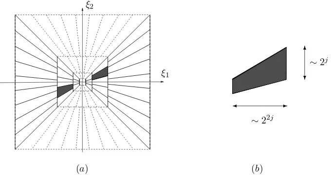
Fig. 1.1. (a)The tiling of the frequency plane R2 induced by the shearlets. (b) Frequency support of the shearletψj,,k, forξ1>0. The other half of the support, forξ1<0, is symmetrical.
construct a Parseval frame (or an orthonormal basis) for L2([−1 8,
1 8]
2)∨. Then any
function in L2(R2) can be expressed as a sum f = P
Cf +PCf +P0f, where each component corresponds to the orthogonal projection of f into one of the three sub-spaces ofL2(R2) described above. The tiling of the frequency planeR2 induced by
this system is illustrated in Figure 1.1(a). The above construction was first introduced in [15].
The conditions on the support of ˆψ1 and ˆψ2imply that the functions ˆψj,,k have frequency support:
supp ˆψj,,k⊂
(ξ1, ξ2) :ξ1∈[−22j−1,−22j−4]∪[22j−4,22j−1],ξ2 ξ1 −2
−j≤2−j
.
Thus, the systemSH(ψ), given by (1.9), is a Parseval frame exhibiting the following properties:
(i) Time-frequency localization. Since ˆψ∈C0∞(R2), then|ψ(x)| ≤C
N(1+|x|)−N for anyN ∈N, and thus the elementsψj,,k are well localized.
(ii) Parabolic scaling. Each element ˆψj,,k has support on a pair of trapezoids, each one contained in a box of size approximately 22j×2j(see Figure 1.1(b)). Because the shearlets are well localized, each ψj,,k is essentially supported on a box of size 2−2j×2−j. Thus, their supports become increasingly thin asj → ∞.
(iii) Directional sensitivity. The elements ˆψj,,kare oriented along lines with slope given by2−j. As a consequence, the corresponding elementsψj,,k are ori-ented along lines with slope −2−j. The number of orientations (approxi-mately) doubles at each finer scale.
(iv) Spatial localization. For any fixed scale and orientation, the shearlets are obtained by translations on the latticeZ2.
(v) Oscillatory behavior. The shearletsψj,,k are nonoscillatory along the orien-tation axis of slope−2−j, and oscillatory across this axis.
orienta-tions in the curvelet construcorienta-tions doubles at every other scale. Concerning property (iv), the curvelets are not associated with afixed translation lattice. However, for a given scale parameterjand orientationθ, they are obtained by translations on a grid that depends on j and θ. In fact, as we mentioned before, unlike the shearlets, the curvelets are not generated from the action of a family of operators on a single or finite family of functions.
1.3. Main results. One major feature of shearlets is that, if f is a compactly supported function which isC2 away from aC2curve, then the sequence of shearlet
coefficients {f, ψj,,k} has (essentially) optimally fast decay. As a consequence, if
fS
N is the N-term approximation of f obtained from the N largest coefficients of its shearlet expansion, then the approximation error is essentially optimal.
Before stating the main theorems, let us define more precisely the class of functions we are interested in. We follow [7] and introduce ST AR2(A), a class of indicator functions of setsB withC2 boundaries∂B. In polar coordinates, letρ(θ) : [0,2π)→ [0,1]2 be a radius function, and define B by x ∈ B if and only if |x| ≤ ρ(θ). In particular, the boundary∂B is given by the curve inR2:
(1.10) β(θ) =
ρ(θ) cos(θ)
ρ(θ) sin(θ)
.
The class of boundaries of interest to us is defined by
(1.11) sup|ρ(θ)| ≤A, ρ≤ρ0<1.
We say that a set B ∈ST AR2(A) if B ⊂[0,1]2 and B is a translate of a set
obey-ing (1.10) and (1.11). In addition, we set C2
0([0,1]2) to be the collection of twice
differentiable functions supported inside [0,1]2.
Finally, we define the set E2(A) of functions which areC2 away from a C2 edge as the collection of functions of the form
f =f0+f1χB,
wheref0, f1∈C02([0,1]2),B∈ST AR2(A), andfC2=
|α|≤2D
αf
∞≤1.
Let M be the set of indices {(j, , k) : j ≥ 0,−2j ≤ ≤ 2j, k ∈ Z2}, and let
{ψμ}μ∈M be the Parseval frame of shearlets given by (1.9). Theshearlet coefficients of a given function f are the elements of the sequence {sμ(f) =f, ψμ: μ ∈ M}. We denote by|s(f)|(N)theNth largest entry in this sequence. We can now state the
following results.
Theorem 1.1. Letf ∈ E2(A), and let{sμ(f) =f, ψμ: μ∈M}be the sequence
of shearlet coefficients associated withf. Then
(1.12) sup
f∈E2(A)|
s(f)|(N)≤C N−3/2(logN)3/2.
LetfNS be theN-term approximation offobtained from theNlargest coefficients of its shearlet expansion, namely,
fNS = μ∈IN
f, ψμψμ,
where IN ⊂ M is the set of indices corresponding to the N largest entries of the sequence{|f, ψμ|2:μ∈M}.Then the approximation error satisfies
f−fNS
2 2≤
m>N
Therefore, from (1.12) we immediately have the following.
Theorem 1.2. Let f ∈ E2(A) andfNS be the approximation tof defined above.
Then
f −fNS22≤C N−2(logN)3.
1.4. Analysis of the shearlet coefficients. The argument that will be used to prove Theorem 1.1 follows essentially the architecture of the proofs in [7]. In order to measure the sparsity of the shearlet coefficients{f, ψμ: μ∈M}, we will use the weak-p quasi-norm·wp defined as follows. Let|sμ|(N)be theNth largest entry in
the sequence{sμ}. Then
sμwp= sup
N >0 N
1
p |s μ|(N).
One can show (cf. [29, sect. 5.3]) that this definition is equivalent to
sμwp=
sup >0
#{μ: |sμ|> }p
1
p
.
To analyze the decay properties of the shearlet coefficients {f, ψμ} at a given scale 2−j, we will smoothly localize the functionf near dyadic squares. Fix the scale parameterj ≥0. For this j fixed, let Mj ={(j, , k) : −2j ≤ ≤ 2j, k ∈Z2} and
Qj be the collection of dyadic cubes of the form Q = [k21j,
k1+1
2j ]×[
k2
2j,
k2+1
2j ], with
k1, k2 ∈ Z. For w a nonnegative C∞ function with support in [−1,1]2, we define a
smooth partition of unity
Q∈Qj
wQ(x) = 1, x∈R2,
where, for each dyadic squareQ∈ Qj,wQ(x) =w(2jx1−k1,2jx2−k2). We will then
examine the shearlet coefficients of the localized functionfQ=f wQ, i.e.,{fQ, ψμ:
μ∈Mj}.
Forf ∈ E2(A), the decay properties of the coefficients{f
Q, ψμ: μ∈Mj} will exhibit a very different behavior depending on whether the edge curve intersects the support ofwQ or not. Let Qj =Qj0∪ Q1j, where the union is disjoint and Q0j is the collection of those dyadic cubesQ∈ Qjsuch that the edge curve intersects the support of wQ. Since each Q has sidelength 2·2−j, thenQ0j has cardinality|Q0j| ≤ C02j, where C0 is independent of j. Similarly, since f is compactly supported in [0,1]2,
|Q1
j| ≤22j+ 4·2j.
We have the following results, which will be proved in section 2.
Theorem 1.3. Let f ∈ E2(A). For Q∈ Q0j, with j ≥ 0 fixed, the sequence of
shearlet coefficients{fQ, ψμ: μ∈Mj} obeys
fQ, ψμw2/3≤C2−
3j
2
for some constant C independent ofQandj.
Theorem 1.4. Let f ∈ E2(A). For Q∈ Q1j, with j ≥ 0 fixed, the sequence of
shearlet coefficients{fQ, ψμ: μ∈Mj} obeys
for some constant C independent ofQandj.
As a consequence of these two theorems, we have the following.
Corollary 1.5. Let f ∈ E2(A) and, for j ≥ 0, let sj(f) be the sequence sj(f) ={f, ψμ: μ∈Mj}. Then
sj(f)w2/3 ≤C
for someC independent of j.
Proof. Using Theorems 1.3 and 1.4, by thep-triangle inequality for weakpspaces,
p≤1, we have
sj(f)
2/3
w2/3 ≤
Q∈Qj
fQ, ψμ
2/3
w2/3
=
Q∈Q0 j
fQ, ψμ
2/3
w2/3+
Q∈Q1 j
fQ, ψμ
2/3
w2/3
≤C|Q0j|2−j+C|Q1j|2−2j.
The proof is completed by observing that|Q0j| ≤C02j, whereC0is independent ofj, and|Q1j| ≤22j+ 4·2j.
We can now prove Theorem 1.1.
Proof of Theorem1.1. By Corollary 1.5, we have that
(1.13) R(j, ) = #{μ∈Mj: |f, ψμ|> } ≤C −2/3.
Also, observe that, since ˆψ∈C0∞(R2), then
|f, ψμ|=
R2
f(x) 23j/2ψ(BAjx−k)dx
≤23j/2f∞
R2
|ψ(BAjx−k)|dx
= 2−3j/2f∞
R2
|ψ(y)|dy < C2−3j/2.
(1.14)
As a consequence, there is a scalejsuch that|f, ψμ|< for eachj ≥j. Specifically, it follows from (1.14) thatR(j, ) = 0 for j >23(log2(−1) + log
2(C))> 2
3 log2(−1).
Thus, using (1.13), we have that
#{μ∈M : |f, ψμ|> } ≤
j≥0
R(j, )≤C −2/3 log2(−1),
and this implies (1.12).
2. Proofs. This section contains the constructions and proofs needed for the theorems in section 1.4.
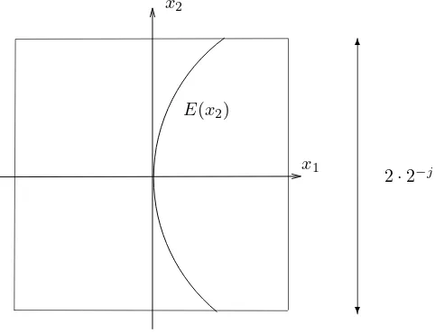
2.1. Proof of Theorem 1.3. Suppose that a function inE2(A) contains aC2
edge. Following the approach in [7], we suppose that, for j > j0, the scale 2−j is
small enough so that over the square −2−j ≤ x
1, x2 ≤ 2−j the edge curve may be
parametrized asE(x2)
x2
or x1
E(x1)
. (The case wherej ≤j0 is small requires a much
x1 x2
E(x2)
6
?
2·2−j
Fig. 2.1.Representation of an edge fragment.
us assume that the first parametrization holds. Then anedge fragment is a function of the form
f(x1, x2) =w(2jx1,2jx2)g(x1, x2)χ{x1≥E(x2)},
where g ∈C02((0,1)2). For simplicity, let us assume that the edge goes through the
origin and, at this point, its tangent is vertical (see Figure 2.1). Then, using the regularity of the edge curve, we have that
(i) E(0) = 0,E(0) = 0;
(ii) sup|x2|≤2−j|E(x2)| ≤ 12 sup|x2|≤2−j2−2j|E(x2)|.
That means that, for|x2| ≤2−j, the edge curve is almost straight. Observe that any
arbitrary edge fragment is obtained by rotating and translating the one above. Since the analysis of the edge fragment that will be presented in the following is not affected by these transformations, there is no loss of generality in considering this case only.
In order to quantify the decay properties of the shearlet coefficients, we first need to analyze the decay of the Fourier transform of the edge fragment along radial lines in the regionDC⊂R2, defined in section 1.2. It will be convenient to introduce polar coordinates. Letξ= (ξ1, ξ2)∈ DC. Using polar coordinates, we have
ξ1=λcosθ, ξ2=λsinθ, with|θ| ≤ π
4, λ∈R,|ξ1| ≥ 1 8.
Using this notation, the radial lines have the form (λcosθ, λsinθ),λ∈R,|θ| ≤ π
4.
Forξ= (ξ1, ξ2)∈ DC,j≥0,−2j ≤≤2j, we introduce the notation
(2.1) Γj,(ξ) = ˆψ1
2−2jξ1 ˆ
ψ2
2j ξ2
ξ1−
.
We have the following claim.
Proposition 2.1. Letf be an edge fragment andΓj, be given by(2.1). Then
R2
|fˆ(ξ)|2|Γ
In order to prove this proposition, we need to recall the following result [7, Thm. 6.1].
Theorem 2.2. Letf be an edge fragment andIj a dyadic interval[22j−α,22j+β]
withα∈ {0,1,2,3,4},β ∈ {0,1,2}. Then, for all θ,
|λ|∈Ij
|fˆ(λcosθ, λsinθ)|2dλ≤C2−3j1 + 2j|sinθ|−5.
Proof of Proposition 2.1. The assumptions on the support of ˆψ1 and ˆψ2 imply
that
(2.2) supp ˆψ1(2−2jξ1) ⊂ ξ1∈[−22j−1,−22j−4]∪[22j−4,22j−1]
and
supp ˆψ2
2jξ2
ξ1 −
⊂
(ξ1, ξ2) :2j ξ2
ξ1 − ≤1
.
Since tanθ=ξ2
ξ1, the last expression can be written as
(2.3) supp ˆψ2
2jξ2
ξ1
−
⊂ (λ, θ) : 2−j(−1)≤tanθ≤2−j(+ 1).
Since λ2 =ξ2
1+ξ22 =ξ21(1 + (tanθ)2) and || ≤ 2j, then, using (2.2) and (2.3), we
have
|λ| ≤22j−1
1 + 2−2j(1 +||)2
1 2
≤22j−1
1 + 2−2j(1 + 2j)2
1 2
≤22j+1
and
|λ| ≥22j−4
1 + 2−2j(|| −1)2
1 2
≥22j−4.
Thus, the support of Γj, is contained in
Wj,={(λ, θ) : 22j−4≤ |λ| ≤22j+1,arctan(2−j(−1))≤θ≤arctan(2−j(+ 1))}.
Observe that, in particular, |θ| ≤arctan 2. Since, for|θ| ≤2, we have that1 tanθ≈
sinθ, it follows from (2.3) that, onWj,,
(2.4) 2j|sinθ| ≈2j(2−j||) =||.
Thus, using (2.4) and Theorem 2.2, we have that
R2
|fˆ(ξ)|2|Γ
j,(ξ)|2dξ ≤C
Wj,
|fˆ(λcosθ, λsinθ)|2λ dλ dθ
≤C
arctan(2−j(+1))
arctan(2−j(−1))
22j+1
22j−4
|fˆ(λcosθ, λsinθ)|2|λ|dλ dθ
≤C22j+1
arctan(2−j(+1))
arctan(2−j(−1))
2−4j
1 + 2j|sinθ| −5
dθ
≤C2−2j(1 +||)−5arctan(2−j(−1))−arctan(2−j(+ 1)) =C2−3j(1 +||)−5.
1We use the notationf(x)≈g(x),x∈D, to mean that there are constantsC
1, C2>0 such that
The following proposition provides a similar estimate for the partial derivatives of the Fourier transform of the edge fragment.
Proposition 2.3. Let f be an edge fragment, Γj, be given by (2.1), andL be
the differential operator
L=
I−
22j 2π(1 +||)
2 ∂2 ∂ξ2
1
1−
2j 2π
2 ∂2 ∂ξ2
2
.
Then
R2
L
ˆ
f(ξ) Γj,(ξ)
2
dξ≤C2−3j(1 +||)−5.
In order to prove this proposition, we need to recall the following result [7, Cor. 6.6].
Corollary 2.4. Letf be an edge fragment andIja dyadic interval[22j−α,22j+β]
with α∈ {0,1,2,3,4},β ∈ {0,1,2}. Then, for each m= (m1, m2)∈N×Nand for
each θ,
|λ|∈Ij
∂m1
∂ξm1
1 ∂m2
∂ξm2
2
ˆ
f(λcosθ, λsinθ)
2 dλ
≤Cm2−2j|m|
2−(4+2m1)j(1 + 2j|sinθ|)−5+ 2−10j
,
whereCm is independent ofj and andN=N∪ {0}.
We also need the following lemma, which follows from a direct computation.
Lemma 2.5. Let Γj, be given by (2.1). Then, for each m= (m1, m2)∈N×N, m1, m2∈ {0,1,2},
∂m1
∂ξm1
1 ∂m2
∂ξm2
2
Γj,(ξ1, ξ2)
≤Cm2−(2m1+m2)j(1 +||)m1,
where|m|=m1+m2 andCmis independent of j and. We can now prove Proposition 2.3.
Proof of Proposition2.3. From Corollary 2.4, using (2.4), we have
22j+1
22j−4
∂ξ∂22
1
ˆ
f(λcosθ, λsinθ)
2
dλ≤C2−4j
2−8j(1 +||)−5+ 2−10j
.
Thus, using the same idea as in the proof of Proposition 2.1,
R2
∂ξ∂22
1
ˆ
f(ξ)
Γj,(ξ)
2 dξ
≤C
arctan(2−j(+1))
arctan(2−j(−1))
22j+1
22j−4
∂ξ∂22
1
ˆ
f(λcosθ, λsinθ)
2
|λ|dλ dθ
≤C2−3j
2−8j(1 +||)−5+ 2−10j
.
Similarly, using Corollary 2.4 and Lemma 2.5, we have R2 ∂ ∂ξ1 ˆ
f(ξ) ∂
∂ξ1
Γj,(ξ)
2 dξ
≤C2−4j(1 +||)2
arctan(2−j(+1))
arctan(2−j(−1))
22j+1
22j−4
∂ξ1∂ fˆ(λcosθ, λsinθ)
2
|λ|dλ dθ
≤C2−4j(1 +||)22−j
2−6j(1 +||)−5+ 2−10j
=C2−5j(1 +||)2
2−6j(1 +||)−5+ 2−10j
(2.6) and R2 fˆ(ξ)
∂2 ∂ξ2
1
Γj,(ξ)
2 dξ
≤C2−8j(1 +||)4
arctan(2−j(+1))
arctan(2−j(−1))
22j+1
22j−4
fˆ(λcosθ, λsinθ)2 |λ|dλ dθ
≤C2−8j(1 +||)42−3j(1 +||)−5=C2−11j(1 +||)−1.
(2.7)
Finally, combining (2.5), (2.6), (2.7), and using the fact that|| ≤2j, we have that
(2.8) R2
22j 2π(1 +||)
2 ∂2 ∂ξ2 1 ˆ
f(ξ) Γj,(ξ)
2
dξ≤C2−3j(1 +||)−5.
Similarly for the derivatives with respect toξ2we have
(2.9) R2 ∂2 ∂ξ2 2 ˆ
f(ξ)
Γj,(ξ)
2dξ≤C2−3j
2−4j(1 +||)−5+ 2−10j
, (2.10) R2 ∂ ∂ξ2 ˆ
f(ξ) ∂
∂ξ2
Γj,(ξ)
2 dξ≤C2−3j
2−4j(1 +||)−5+ 2−10j
, (2.11) R2 fˆ(ξ)
∂2 ∂ξ2
2
Γj,(ξ)
2dξ ≤C2−7j(1 +||)−5.
Combining (2.9), (2.10), (2.11), and using again the fact that|| ≤2j, we have that
(2.12) R2 2j 2π 2 ∂2 ∂ξ2 2 ˆ
f(ξ) Γj,(ξ)
2
dξ≤C2−3j(1 +||)−5.
Similarly, one can show that
(2.13)
R2
(1 +|23|)(2j π)2 ∂2 ∂ξ2 2 ∂2 ∂ξ2 1 ˆ
f(ξ) Γj,(ξ)
2 dξ≤C2−3j(1 +||)−5.
The proof is completed using (2.8), (2.12), (2.13), and Lemma 2.5.
Proof of Theorem1.3. Fix j≥0 and, for simplicity of notation, letf =fQ. For
μ∈Mj, the shearlet coefficient off is
f, ψμ=f, ψj,,k=|detA|−j/2
R2
ˆ
f(ξ) Γj,(ξ)e2πiξA −jB−k
dξ,
where Γj,(ξ) is given by (2.1) andA,B are given by (1.4). Observe that
2πiξA−jB−k= 2πiξ1 ξ2 2− 2j 0 0 2−j
1 −
0 1
k1 k2
= 2πi(k1−k2)2−2jξ1+k22−jξ2.
(2.14)
Using (2.14), a direct computation shows that
∂2 ∂ξ2
1
2πξA−jB−k=−(2π)22−4j(k1−k2)2=
−(2π)222−4j(k1
−k2)2 if= 0,
−(2π)22−4jk21 if= 0,
∂2 ∂ξ2
2
2πξA−jB−k=−(2π)22−2jk22.
(2.15)
By the equivalent definition of weakp norm, the theorem is proved, provided we show that
(2.16) #{μ∈Mj : |f, ψμ|> } ≤C2−j−
2 3.
LetLbe the second order differential operator defined in Proposition 2.3. Using (2.14) and (2.15), it follows that
(2.17)
Le2πiξA−jB−k=
⎧ ⎨ ⎩
1 +
(1+||) 2
k1
−k2
2
(1 +k22)e2πiξA
−jB−k
if= 0,
(1 +k2
1)(1 +k22)e2πiξA
−jB−k
if= 0.
Integration by parts gives
f, ψμ=|detA|−j/2
R2
L
ˆ
f(ξ) Γj,(ξ)
L−1
e2πiξA−jB−k
dξ.
Let us consider first the case= 0. In this case, from (2.17) we have that
(2.18) L−1e2πiξA−jB−k=G(k, )−1e2πiξA−jB−k,
whereG(k, ) =1 +(1+||)2k1
−k2
2
(1 +k22). Thus
f, ψμ=|detA|−j/2G(k, )−1
R2
L
ˆ
f(ξ) Γj,(ξ)
e2πiξA−jB−kdξ,
or, equivalently,
G(k, )f, ψμ=|detA|−j/2
R2
L
ˆ
f(ξ) Γj,(ξ)
e2πiξA−jB−kdξ.
LetK= (K1, K2)∈Z2, and defineRK ={k= (k1, k2)∈Z2: k1 ∈[K1, K1+1], k2= K2}. Since, forj, fixed, the set{|detA|−j/2e2πiξA
−jB−k
basis for theL2 functions on [−1 2,
1 2]A
jB, and the function Γ
j,(ξ) is supported on this set, then
k∈RK
|G(k, )f, ψμ|2≤
R2
L
ˆ
f(ξ) Γj,(ξ)
2 dξ.
From the definition ofRK it follows that
k∈RK
|f, ψμ|2≤C
1 + (K1−K2)2−2(1 +K2)−2
R2
L
ˆ
f(ξ) Γj,(ξ)
2 dξ.
By Proposition 2.3,
(2.19)
k∈RK
|f, ψμ|2≤C L−K22−
3j(1 +||)−5,
where LK = (1 + (K1−K2)2)(1 +K22). For j, fixed, letNj,,K() = #{k ∈RK :
|ψj,,k|> }. Then it is clear thatNj,,K()≤C(||+ 1), and (2.19) implies that
Nj,,K()≤C L−K22−
3j−2(1 +||)−5.
Thus
(2.20) Nj,,K()≤C min
||+ 1, L−K22−3j−2(1 +||)−5.
Using (2.20), we will now show that
(2.21)
2j
=−2j
Nj,,K()≤C L
−23
K 2− j−23.
In fact, let ∗ be defined by (∗+ 1) = L−K22−3j−2(1 +∗)−5. That is, ∗+ 1 = L−K1/32−j/2−1/3.Then
2j
=−2j
Nj,,K()≤
||≤(∗+1)
Nj,,K() +
||>(∗+1)
Nj,,K()
≤
||≤(∗+1)
(||+ 1) +
||>(∗+1)
L−K22−3j−2(1 +||)−5
≤(∗+ 1)2+C L−K22−3j−2(1 +∗)−4≤C(∗+ 1)2,
which gives (2.21). SinceK∈Z2L−
2/3
K <∞, using (2.21) we then have that
#{μ∈Mj: |f, ψμ|> } ≤
K∈Z2
2j
=−2j
Nj,,K()≤C2−j−
2
3
K∈Z2
L− 2 3
K ≤C2−
j−23,
and, thus (2.16) holds.
The case= 0 is similar. Indeed, in this case
L−1e2πiξA−jB−k= (1 +k12)−1(1 +k22)−1e2πiξA−jB−k,
and we can proceed as in the case= 0, withLK = (1 +K12) (1 +K22). It is clear that
also in this caseK∈Z2L−
2/3
2.2. Proof of Theorem 1.4. In order to prove Theorem 1.4, the following lemmata will be useful.
Lemma 2.6. Let f =g wQ, whereg∈ E2(A)andQ∈ Q1j. Then
(2.22)
Wj,
|fˆ(ξ)|2dξ≤C2−10j.
Proof. The proof follows [7, Lem. 8.1] and is reported here for completeness. The functionf belongs toC2
0(R2), and its second partial derivative with respect
tox1is
∂2f ∂x2 1
= ∂
2g ∂x2 1
wQ+ 2
∂ g ∂x1
∂ wQ
∂x1 +f ∂2wQ
∂x2 1
=h1+h2+h3.
Using the fact thatwQ is supported in a square of sidelength 2·2−j, we have
R2
|ˆh1(ξ)|2dξ=
R2
|h1(x)|2 dx≤C2−2j.
Next, observe that∂x∂
1h2∞≤C2
2j. Using again the condition on the support of
wQ, it follows that
R2
|2πξ1ˆh2(ξ)|2dξ=
R2
∂
∂x1 h2(x)
2
dx≤C22j,
and thus, forξ∈Wj, (henceξ1≈22j),
Wj,
|ˆh
2(ξ)|2dξ≤C2−2j.
Finally, observing that ∂x∂22 1
h3∞ ≤ C24j, a computation similar to the one above
shows that
Wj,
|ˆh3(ξ)|2dξ≤C2−2j.
Since−(2π)2ξ2
1fˆ(ξ) = ˆh1(ξ) + ˆh2(ξ) + ˆh3(ξ),it follows from the estimates above that
Wj,
|fˆ(ξ)|2dξ≤C2−10j.
This completes the proof.
Lemma 2.7. Let m= (m1, m2)∈N×N,ξ= (ξ1, ξ2)∈R2, and Γj, be given by
(2.1). Then
2j
=−2j
∂m1
∂ξm1
1 ∂m2
∂ξm2
2
Γj,(ξ)
2≤Cm2−2|m|j,
whereCm is independent ofj andξ and|m|=m1+m2.
Lemma 2.8. Let f =g wQ, whereg∈ E2(A)andQ∈ Q1j. Define
(2.23) T =
I− 2
j
(2π)2Δ
,
whereΔ = ∂ξ∂22 1
+∂ξ∂22 2 . Then R2 2j
=−2j
T2
ˆ
fΓj,
(ξ)
2
dξ≤C2−10j.
Proof. Observe that, forN ∈N,
ΔN
ˆ
fΓj,
=
|α|+|β|=2N
Cα,β
∂α1
∂ξα1
1 ∂α2
∂ξα2
2
ˆ
f ∂
β1
∂ξβ1
1 ∂β2
∂ξβ2
2
Γj,
.
Then, using Lemma 2.7, we have that
R2
2j
=−2j
∂α1
∂ξα1
1 ∂α2
∂ξα2
2
ˆ
f(ξ)
2
∂β1
∂ξβ1
1 ∂β2
∂ξβ2
2
Γj,(ξ)
2
dξ
≤Cβ2−2|β|j
Wj,
∂α1
∂ξα1
1 ∂α2
∂ξα2
2
ˆ
f(ξ)
2 dξ.
Recall thatf(x) is of the formg(x)w(2jx). It follows thatxαf(x) = 2−j|α|g(x)w α(2jx), where wα(x) = xαw(x). By Lemma 2.6, g(x)wα(2jx) obeys the estimate (2.22). Thus, observing that ∂ξ∂αα11
1
∂α2
∂ξα2 2
ˆ
f(ξ) is the Fourier transform of (−2πix)αf(x), we have that
Wj,
∂α1
∂ξα1
1 ∂α2
∂ξα2
2
ˆ
f(ξ)
2
dξ≤Cα2−2j|α|2−10j.
Combining the estimates above, we have that, for eachα, β with|α|+|β|= 2N,
(2.24)
R2
2j
=−2j
∂α1
∂ξα1
1 ∂α2
∂ξα2
2
ˆ
f(ξ)
2
∂β1
∂ξβ1
1 ∂β2
∂ξβ2
2
Γj,(ξ)
2
dξ≤Cα,β2−10j2−4jN.
SinceT2= 1−2 2j
(2π)2Δ +
22j
(2π)4Δ2, the lemma now follows from (2.24) and Lemma
2.7.
We can now prove Theorem 1.4.
Proof of Theorem1.4. Using (2.15), forT given by (2.23), we have that
(2.25) Te2πiξA−jB−k=1 + 2−2j(k1−k2)2+k22
e2πiξA−jB−k.
Fix j ≥0 and let f =fQ. Then, using integration by parts as in the proof of Theorem 1.3, from (2.25) it follows that
f, ψμ=|detA|−j
1 + 2−2j(k1−k2)2+k22−2
R2
T2
ˆ
fΓj,
LetK= (K1, K2)∈Z2andR
K be the set {(k1, k2)∈Z2:k2=K2,2−j(k1−K2)∈ [K1, K1+ 1]}. Observing that, for eachK, there are only 1 + 2j choices fork1inR
K, it follows that the number of terms inRK is bounded by 1 + 2j. Thus, arguing again as in the proof of Theorem 1.3, we have that
k∈RK
|f, ψμ|2≤C
1 +K12+K 2 2
−4
R2
T2
ˆ
fΓj,
(ξ)
2 dξ.
From this inequality, using Lemma 2.8, we have that
2j
=−2j
k∈RK
|f, ψμ|2≤C(1 +K2)−4
R2
2j
=−2j
T2
ˆ
fΓj,
(ξ)
2 dξ
≤C(1 +K2)−42−10j.
(2.26)
For anyN ∈N, provided 1
2 < p <2, the H¨older inequality yields
(2.27)
N
m=1
|am|p≤
N
m=1
|am|2
p
2 N
1−p
2
.
Since the cardinality of RK is bounded by 1 + 2j, it follows from (2.26) and (2.27) that, for 1
2 < p <2,
2j
=−2j
k∈RK
|f, ψμ|p≤C
22j(1− p
2)(1 +K2)−2p2−5pj.
Thus, sincep > 12,
μ∈Mj
|f, ψμ|p≤C2
2j(1−p2)−5pj
K∈Z2
(1 +K2)−2p≤C2(2−3p)j,
and, in particular,
f, ψμ2/3≤C2−3j.
2.3. Coarse scale analysis. In section 2.1, we assumed that the scale parameter
j was large enough. The situation wherej is small can be treated in a much simpler way. In fact, iffQ is an edge fragment, then a trivial estimate shows that
fQ2=
suppwQ
|fQ(x)|2dx
1/2
≤C|suppwQ|=C2−j.
It follows thatfQ, ψμ2 ≤C2−j, and thus, by the H¨older inequality,
fQ, ψμ2/3 ≤C2j.
2.4. Additional remarks.
• In order to define the collection of shearlets, in section 1.2 we have constructed a function ˆψ∈C0∞. This property allows us to obtain a collection of elements that are well localized. Observe, however, that we need only ˆψ∈C02in order
to prove all the results presented in this paper.
• In this paper, we have considered the representation of functions containing a discontinuity along aC2curve. More generally, we can consider the situation
where a functionf contains many edge curves of this type, exhibiting finitely many junctions or corners between them. In this setting, the discontinuity curve is not globally C2 but only piecewiseC2. The results reported in this
paper, namely Theorems 1.1 and 1.2, extend to this setting as well. We refer to [7] for a similar discussion in the case of curvelets.
• The assumption we made about the regularity of the discontinuity curve plays a critical role in our construction. If the discontinuity curve is in Cα, with
α > 2, then our argument still works and we can still prove Theorem 1.2. This result, however, is not (essentially) optimal as in the caseα= 2. On the other hand, if the discontinuity curve is inCα, withα <2, then the estimate given by Theorem 1.2 does not hold, and the estimate could be worse in general. We refer to [24] for additional observations about this fact, and for an alternative approach, based on an adaptive construction, to the sparse representation of functions with edges.
• There are natural ways of extending the shearlets to dimensions larger than 2. We refer to [18] for a discussion of these extensions, as well as the extensions of the shear transformations to the general multidimensional setting. For example, in dimension 3, let A =40 20I2; define the shear matrices {Sk =
1 k 0I2
: k ∈ Z2}, where I2 is the 2×2 identity matrix, 0 = (0
0); and, for ξ= (ξ1, ξ2, ξ3)∈R3, defineψby
ˆ
ψ(ξ) = ˆψ1(ξ1) ˆψ2
ξ2 ξ1
ˆ
ψ2
ξ3 ξ1
,
where ψ1 and ψ2 are given as in the 2-D case. Then, similarly to their 2-D
counterpart, one can construct a Parseval frame of well-localized 3-D shearlets
{ψj,,k =|detA|−j/2ψ(SA−jx−k) : j∈Z, ∈Z2, k∈Z2},
with frequency support on a parallelepiped of approximate size 22j×2j × 2j, at various scales j, with orientations controlled by the 2-D index and spatial locationk. Then, using a heuristic argument, one can argue that these systems provide sparse representations for 3-D functionsf that are smooth away from “nice” surface discontinuities of finite area. In fact, thanks to their frequency support and their localization properties, the elementsψj,,k, at scalej, are essentially supported on a parallelepiped of size 2−2j×2−j×2−j, with location controlled bykand orientation controlled by. Thus, there are at most O(22j) significant shearlet coefficients SH
j,,k(f) =f, ψj,,k, and they are bounded byC2−2j. This implies that the Nth largest 3-D shearlet coefficient|SHN(f)|is bounded byO(N−1), and thus, iff is approximated by taking theN largest coefficients in the 3-D shearlets expansion, theL2-error
would approximately obey
f−fNS2L2 ≤
>N
up to lower order factors. A rigorous proof of this fact will be presented elsewhere.
Appendix. Construction ofψ1, ψ2. In this section we show how to construct
examples of functionsψ1,ψ2 satisfying the properties described in section 1.2. In order to constructψ1, leth(t) be an evenC0∞function, with support in (−16,16), satisfyingRh(t)dt = π2, and define θ(ω) = −∞ω h(t)dt. Then one can construct a smooth bell function as
b(ω) =
⎧ ⎪ ⎪ ⎨ ⎪ ⎪ ⎩
sinθ|ω| − 12 if 13 ≤ |ω| ≤ 23,
sin
π
2 −θ
|ω|
2 − 1 2
if 23 <|ω| ≤ 43,
0 otherwise.
It follows from our assumptions (cf. [20, sect. 1.4]) that
∞
j=−1
b2(2−jω) = 1 for|ω| ≥ 1
3.
Now lettingu2(ω) =b2(2ω) +b2(ω), it follows that
∞
j≥0
u2(2−2jω) =
∞
j=−1
b2(2−jω) = 1 for|ω| ≥ 1
3.
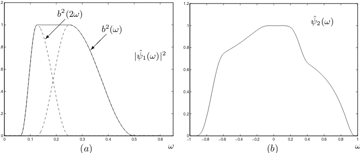
Finally, letψ1 be defined by ˆψ1(ω) =u(83ω).Then supp ˆψ1⊂[−12,−161]∪[161,12], and (1.6) is satisfied. This construction is illustrated in Figure A.1(a).
0 0.1 0.2 0.3 0.4 0.5 0.6 0
0.2 0.4 0.6 0.8 1 1.2
−1 −0.8 −0.6 −0.4 −0.2 0 0.2 0.4 0.6 0.8 1 0
0.2 0.4 0.6 0.8 1 1.2
(a) ω
b2(ω) b2(2ω)
|ψˆ1(ω)|2
(b) ω
ˆ ψ2(ω)
Fig. A.1. (a)The function|ψˆ1(ω)|2 (solid line), for ω >0; the negative side is symmetrical. This function is obtained, after rescaling, from the sum of the window functions b2(ω) +b2(2ω) (dashed lines). (b)The functionψˆ2(ω).
For the construction ofψ2, we start by considering a smooth bump functionf1∈ C0∞(−1, 1) such that 0≤f1≤1 on (−1,1) andf1= 1 on [−12,12] (cf. [21, sect. 1.4]). Next, letf2(t) = 1−exp (1/t). Then (in the left limit sense)f2(0) = 1, f
(k) 2 (0) = 0
for k ≥1 and 0< f2 <1 on (−1,0). Define f(t) = f1(t)f2(t) fort ∈ [−1,0]. It is
Sinceg(t) = exp (2(t1−1)) for t∈(12,1), it follows that limt→1−g(k)(t) = 0 fork≥0.
Finally, we define
ˆ
ψ2(ω) = ⎧ ⎪ ⎨ ⎪ ⎩
f(ω) ifω∈[−1,0),
g(ω) ifω∈[0,1],
0 otherwise.
Then ˆψ2∈C0∞(R), with supp ˆψ2⊂[−1,1], and
ˆ
ψ22(ω) + ˆψ22(ω−1) = 1, ω∈[0,1].
The last equality implies (1.7). The function ˆψ2 is illustrated in Figure A.1(b).
Acknowledgments. The authors thank E. Cand`es, P. Gremaud, G. Kutyniok, W. Lim, G. Weiss, and E. Wilson for useful discussions.
REFERENCES
[1] J. P. Antoine, R. Murenzi, and P. Vandergheynst,Directional wavelets revisited: Cauchy wavelets and symmetry detection in patterns, Appl. Comput. Harmon. Anal., 6 (1999), pp. 314–345.
[2] R. H. Bamberger and M. J. T. Smith,A filter bank for directional decomposition of images: Theory and design, IEEE Trans. Signal Process., 40 (1992), pp. 882–893.
[3] C. M. Brislawn,Fingerprints go digital, Notices Amer. Math. Soc., 42 (1995), pp. 1278–1283.
[4] C. M. Brislawn and M. D. Quirk, Image compression with the JPEG-2000 standard, in
Encyclopedia of Optical Engineering, R. G. Driggers, ed., Marcel Dekker, New York, 2003, pp. 780–785.
[5] E. J. Cand`es and D. L. Donoho,Ridgelets: A key to higher-dimensional intermittency?,
Phil. Trans. Royal Soc. London A, 357 (1999), pp. 2495–2509.
[6] E. J. Cand`es and D. L. Donoho,Curvelets—A surprising effective nonadaptive representation for objects with edges, in Curves and Surfaces, C. Rabut, A. Cohen, and L. L. Schumaker, eds., Vanderbilt University Press, Nashville, TN, 2000.
[7] E. J. Cand`es and D. L. Donoho,New tight frames of curvelets and optimal representations of objects with piecewiseC2 singularities, Comm. Pure Appl. Math., 56 (2004), pp. 216–266. [8] R. R. Coifman and F. G. Meyer,Brushlets: A tool for directional image analysis and image
compression, Appl. Comput. Harmonic Anal., 5 (1997), pp. 147–187.
[9] S. Dahlke, G. Kutyniok, P. Maass, C. Sagiv, and H.-G. Stark,The Uncertainty Principle Associated with the Continuous Shearlet Transform, preprint, 2006.
[10] R. A. DeVore,Nonlinear approximation, in Acta Numerica, A. Iserles, ed., Cambridge
Uni-versity Press, Cambridge, UK, 1998, pp. 51–150.
[11] M. N. Do and M. Vetterli,The contourlet transform: An efficient directional multiresolution image representation, IEEE Trans. Image Process., 14 (2005), pp. 2091–2106.
[12] D. L. Donoho, Sparse components of images and optimal atomic decomposition, Constr.
Approx., 17 (2001), pp. 353–382.
[13] D. L. Donoho, M. Vetterli, R. A. DeVore, and I. Daubechies, Data compression and harmonic analysis, IEEE Trans. Inform. Theory, 44 (1998), pp. 2435–2476.
[14] G. Easley, D. Labate, and W.-Q. Lim,Sparse Directional Image Representations Using the Discrete Shearlet Transform, preprint, 2006.
[15] K. Guo, G. Kutyniok, and D. Labate, Sparse multidimensional representations using anisotropic dilation and shear operators,in Wavelets and Splines, G. Chen and M. Lai, eds., Nashboro Press, Nashville, TN, 2006, pp. 189–201.
[16] K. Guo, W.-Q. Lim, D. Labate, G. Weiss, and E. Wilson,Wavelets with composite dilations,
Electron. Res. Announc. Amer. Math. Soc., 10 (2004), pp. 78–87.
[17] K. Guo, W.-Q. Lim, D. Labate, G. Weiss, and E. Wilson,The theory of wavelets with com-posite dilations, in Harmonic Analysis and Applications, C. Heil, ed., Birkh¨auser Boston, Cambridge, MA, 2006, pp. 231–249.