DOI: 10.1534/genetics.109.113183
Bayesian Quantitative Trait Locus Mapping Using Inferred Haplotypes
Caroline Durrant
1and Richard Mott
Wellcome Trust Centre for Human Genetics, University of Oxford, Oxford, OX3 7BN, United Kingdom Manuscript received December 16, 2009
Accepted for publication December 23, 2009
ABSTRACT
We describe a fast hierarchical Bayesian method for mapping quantitative trait loci by haplotype-based association, applicable when haplotypes are not observed directly but are inferred from multiple marker genotypes. The method avoids the use of a Monte Carlo Markov chain by employing priors for which the likelihood factorizes completely. It is parameterized by a single hyperparameter, the fraction of variance explained by the quantitative trait locus, compared to the frequentist fixed-effects model, which requires a parameter for the phenotypic effect of each combination of haplotypes; nevertheless it still provides estimates of haplotype effects. We use simulation to show that the method matches the power of the frequentist regression model and, when the haplotypes are inferred, exceeds it for small QTL effect sizes. The Bayesian estimates of the haplotype effects are more accurate than the frequentist estimates, for both known and inferred haplotypes, which indicates that this advantage is independent of the effect of uncertainty in haplotype inference and will hold in comparison with frequentist methods in general. We apply the method to data from a panel of recombinant inbred lines ofArabidopsis thaliana, descended from 19 inbred founders.
A
S the power of haplotypic association has become better appreciated, studies using inferred multi-allelic loci (i.e., haplotypes or pairs of haplotypes) are be-coming more common. This is because single-nucleotide polymorphisms (SNPs), which are the most commonly used type of marker, are very susceptible to a loss of power to detect QTL, due to a mismatch in allele frequencies between the SNP and the causative variant. While multi-allelic markers contain more information and have greater power than SNPs for QTL mapping, they are more costly and cumbersome. Consequently a major analytical ad-vance has been the combination of multiple SNP marker information, either to infer haplotypes as in many human association studies or to infer the mosaic of ancestral founder haplotypes in synthetic populations descended from multiple founder strains. The latter scenario in-cludes crosses between inbred strains of mice or rats or inbred accessions of plants.However, there are two potential difficulties with haplotypic association. First, in a fixed-effects frame-work, a parameter is estimated for each haplotype, which is undesirable when the number of haplotypes is large. In a synthetic population descended from N inbred strains, up toNhaplotypes may segregate; for the mouse collaborative cross (Threadgillet al.2002)N¼8 and
for theArabidopsis thalianamultiparent advanced
gen-eration intercross (MAGIC) population of recombinant inbred lines,N¼19 (Koveret al.2009). For complex
traits, where many QTL are expected to segregate, mul-tiple QTL mapping only exacerbates problems with the numbers of parameters.
Second, one must account for uncertainty in the in-ference of haplotypes, which depends on the marker density and how well one can distinguish between all founders at a locus. At some loci the founders’ hap-lotypes may be identical, for example, in crosses de-scended from inbred strains of mice.
These problems are well known in haplotype associ-ation mapping involving human populassoci-ations, where in general fixed-effects regression modeling is used. Con-sequently methods have been developed to reduce the number of haplotype groups at a marker locus, using hierarchical clustering and Bayesian partitioning algo-rithms (Molitor et al. 2003; Durrant et al. 2004;
Bardel et al. 2006; Morris 2006; Tzeng et al. 2006;
Waldronet al. 2006; Igo et al. 2007; Liu et al. 2007;
Tachmazidouet al.2007; Knightet al.2008).
Bayesian methods are increasingly the approach of choice for QTL mapping, particularly for multiple QTL mapping and the modeling of interactions (Yi and
Shriner 2008). The hierarchical Bayesian framework
can accommodate more complicated models with more parameters, even when there are many more parameters than observations (Meuwissen et al. 2001; Xu 2003).
The Bayesian approach has an additional advantage when the inferred haplotypes are not all identifiable. Reliable estimates of haplotype effects can be determined because the shrinkage effect of the prior distribution Supporting information is available online athttp://www.genetics.org/
cgi/content/full/genetics.109.113183/DC1.
1Corresponding author:Wellcome Trust Centre for Human Genetics,
Roosevelt Dr., Headington, Oxford OX3 7BN, United Kingdom. E-mail: [email protected]
restricts the posterior. However, these methods must be fast if these complex analyses are to be practical.
In a hierarchical model the key problem is how to model the distribution of the variance attributable to a QTL and its prior. Meuwissen et al.(2001) consider a
hierarchical Bayesian random-effects model (HBREM) for observed multiallelic marker loci. They choose nor-mal priors centered at zero for the individual genotype effects, with different variances for each locus. The prior distributions for the variance parameters are scaled inverse chi square, with parameters chosen to give the mean and variance preestimated from the data. However, this prior has a tiny probability of a QTL effect being equal to zero, whereas that is clearly very likely in a genome scan. Hence they also showed an alternative prior, a mixture of a point mass at zero and a scaled inverse chi-square distribution, which gave better results.
Xu(2003) considers a noninformative Jeffrey’s prior
on the locus variance. The model fits all markers si-multaneously and can detect large-effect QTL with little noise at other markers, despite the negligible probabil-ity of zero locus variance. However, the model is limited to markers with two or three possible genotypes. Wang et al.(2005) extend this approach to inferred genotypes, but still with only two or three possible genotypes per locus and the method is very computationally intensive. Yi and Xu (2008) argue that the noninformative
Jeffrey’s prior on the locus variance induces constant shrinkage on the haplotype effects and that it would be preferable to vary shrinkage according to the data. They compare exponential and scaled inverse chi-square priors on the locus variance, using hyperparameters with vague hyperpriors. They also consider a second prior on the haplotype effects (first proposed by Park
and Casella2008), of a normal distribution with
var-iance proportional to the residual error varvar-iance. The four models performed equally when tested on popula-tions with only two genotypes segregating at a locus.
There are several frequentist approaches to dealing with haplotype uncertainty in QTL mapping. One is to perform a fixed-effects multiple linear regression or generalized linear regression of the phenotype, treating the haplotype probabilities at the locus as the design matrix (Haley and Knott 1992; Mott et al. 2000).
Another is to use multiple imputation to draw samples of haplotypes from the haplotype probabilities (Senand
Churchill2001). A third is to use the EM algorithm
to estimate the haplotypes (Excoffier and Slatkin
1995; Hawleyand Kidd1995; Longet al.1995; Qinet al.
2002; Linet al. 2005, 2008; Lin and Zeng2006; Zeng et al.2006). An alternative is data expansion, where in-stead of multiple imputation, the data set is expanded by drawing 10–20 replicate haplotype pairs for every indi-vidual from their inferred probability distribution, assign-ing the same value of the response variable to each, and analyzing the expanded data set. However, this may alter
the characteristics of the data, such as the haplotype frequencies.
In a Bayesian setting, haplotype uncertainty can be accommodated either by including the predictor varia-bles as unknowns in the updating procedure or by multiple imputation. In a fully Bayesian treatment, the unknown haplotype pair assignments are assigned priors and estimated along with the model parameters. However, Markov chain Monte Carlo (MCMC) is then needed to fit the model, updating the parameters on the basis of the haplotype pairs and then updating the haplotype pairs on the basis of the parameters. Updat-ing the haplotype assignments by MCMC is slow and suffers from the label-switching problem among others ( Jasraet al.2005), so an alternative approach would be
preferable.
In this article, we present a new HBREM for QTL mapping applicable to observed or inferred haplotypes. It does not require costly MCMC techniques, since the joint posterior distribution factorizes. It parameterizes the variance terms in the model, focusing on the pro-portion of the variance due to the QTL. We compare its performance with that of the frequentist fixed-effects model for both observed and inferred multiallelic loci. We show first that the posterior mode of the proportion of variance due to a locus is a better outcome measure than two standard Bayesian test statistics and second that the Bayesian estimates of the individual haplotype effects are much more accurate than the corresponding frequentist estimates. Finally we analyze real data from
A. thaliana recombinant inbred lines descended from 19 parental lines.
METHODS
Model:To be as general as possible, we use a notation for modeling the haplotypic effects that applies equally to an outbred diploid population (e.g., humans) in which two distinct haplotypes are present in an in-dividual, givingKhaplotype pairs, and a population of recombinant inbred lines (RIL) in which only one distinct haplotype is present in an individual, givingK
haplotypes. Therefore ‘‘haplotype pair’’ should be read as ‘‘haplotype’’ in the case of RILs. We model a single locus at a time for direct comparison with the frequentist fixed effects model, although the extension to a multi-locus model may be more relevant for many data sets.
Consider a locus whereKhaplotype pairs segregate. We first assume the haplotypes are known and then generalize to the more common situation where they are inferred, as is the case whenever only unphased SNP data are available or when the number of haplotypes is larger than the number of SNP alleles.
is left to the user. In human populations, PHASE is commonly used (Stephenset al.2001; Liand Stephens
2003; Stephens and Donnelly 2003). In synthetic
animal and plant populations descended from known inbred strains the probability of descent from each an-cestral haplotype can be estimated by a hidden Markov model (HMM) (Mottet al.2000).
For a continuously distributed trait and known hap-lotype pairs, the observed phenotypic value yn for in-dividualnis described by the linear regression model
yn ¼m1xnT1en; n¼1;2;. . . ;N;
wheremis the phenotypic mean,T¼[T1,. . .,TK] is the
vector of effect parameters for the haplotype pairs at the locus such thatPKk¼1Tk¼0, andxn¼[xn1,. . .,xnK],n¼ 1, 2,. . .,Nare indicator vectors, such that for individual
nwith haplotype pairm,xnm¼1 andxnk¼0,k6¼m. The residual error terms
en N½0;ð1kÞs2; n ¼1;2;. . .;N;
wheres2is the total phenotypic variance andke[0, 1] is
the proportion of the total phenotypic variance due to the locus. In the case of diploid populations we fit haplotype pairs rather than individual haplotypes to allow for nonadditive effects.
Multiple imputation has traditionally been used when only a small fraction of the genotype data are missing. Complete data sets are created by sampling the missing genotypes from their probability distribution. But for inferred haplotypes, all of the data are missing and there are very many possible data sets, each with small probability. Therefore, imputing from a small number of sampled data sets is unlikely to sample the space adequately. However, since the probability distribution pnis known, instead we sample data sets of haplotype pairs from this distribution, drawing a new haplotype pair for each individual each time a draw of the model parameters is made. This averages the distributions of the parameters over a wide range of possible data sets and effectively treats the inferred haplotype pair prob-abilities as a posterior distribution rather than a prior in the MCMC method. In some situations updating the haplotypes in a fully Bayesian way would be better, but it is computationally intensive and any advantage gained depends on the quality of the prior. If the prior estimates of the haplotype probabilities are accurate, then little benefit would be gained by updating them in the model. We use multiple imputation, sampling haplotype pairs from the probabilitiespn. We assume the haplotype pairs do not depend on the model parameters or the phe-notype. This is certainly reasonable for the majority of loci, since the phenotype depends only on genotypes at QTL, which will not be true for most loci for any given phenotype. We also assume that individuals are unre-lated and hence that their haplotype distributions are independent, as for standard association mapping.
Prior distributions: We choose uninformative priors for the parameters. The phenotypic meanmcould take any real value and the total variances2could take any
positive real value, and these values would not necessar-ily depend on each other. Hencemands2were assumed
to be independent, such that p(m)}1 for me(–‘, ‘) (the location-invariant Jeffrey’s prior for the normal distribution) and s2 Inv – x2[n ¼ 0] (the
scale-invariant Jeffrey’s prior for a variance with degrees of freedomn).
The phenotypic effect parametersTk,k¼1,. . .,Kfor the haplotype pairs are draws from a distribution that could take any real value and should ideally sum to zero over the sample because they are deviations from the overall mean. This may not apply in individual samples of data, however, since the sample frequencies of the haplotype pairs will vary, and it would also lead to de-pendency between the parameters. Instead, a weaker condition is imposed in the prior, thatE(Tk)¼0. The
prior distribution of the effect parameters was chosen to follow a normal distribution, the distribution with the greatest entropy, which must have variance ks2by
the definition ofk,
Tjs2; k Y
K
k¼1
NðTkj0;ks2Þ:
The proportion of variance k due to the effect of the locus is the main parameter of interest. The pro-portion at any particular locus has a high prior of being at or near zero, but with the possibility of being very large. Thus the natural choice of prior for a proportion would appear to be a Beta(a,b) distribution. However, when we implemented this prior for the single-locus model, the posterior distribution ofkwas found to be highly sensitive to the choice of the hyperparameters
a,b(data not shown). Therefore the hyperparameters would need to be included in an additional level of the hierarchical model and estimated simultaneously from the data, following the approach of Yiand Xu(2008).
Moreover, such a prior onkwould shrink the estimates of smaller effects and potentially reduce power to detect them.
Ideally k should give an accurate estimate of the proportion of phenotypic variance due to the locus, large or small. Hence we choose a flat, noninformative prior
pðkÞ Unif½0;1;
Posterior computation:Conditional on the haplotype pairs, the joint posterior distributionp(T,m,s2,kjy,X)
can be factorized completely,
pðT;m;s2;kjy;XÞ
¼ Y
K
k¼1
pðTkjm;s2;k;y;XÞ
" #
pðmjs2;k;y;XÞpðs2 jk;y;XÞpðkjy;XÞ; ð1Þ
whereXis theNxKmatrix with rows corresponding to the indicator vectorsxn. (The derivation of this result follows the factorization of a similar model, which could also be used for this problem, in Chap. 5, section 5.4 of Gelmanet al.2004, and is given in full in theappendix.)
The conditional posterior distributions of the parame-ters are calculated by integrating the joint posterior. First define lk[1=k1ð1kÞ=Nk and L[
PK k¼1lk.
Then we find
pðTkjm;s2;k;y;XÞ N klkðykmÞ;klk
ð1kÞ
Nk s2 ; ð2Þ
pðmjs2;k;y;XÞ N
PK k¼1lkyk
L ;
s2 L
; ð3Þ
pðs2jk;y;XÞ Scaled Invx2½ðN 1Þ;r2; where
r2¼ 1 ðN 1Þ
XN
n¼1
yn2kX
K
k¼1
lkNky2k ð1kÞ
ðPK k¼1lkykÞ2
L
" #
and
pðkjy;XÞ}ð1kÞðK1Þ=2L1=2 Y
K
k¼1
lk
" #1=2
rðN1Þ;
whereNkis the number of individuals with haplotype pairkandyk¼ ð1=NkÞ
PNk
n¼1yknis the mean phenotypic
value for haplotype pairk.
The factorization (1) can be used to make a series of draws numberedd¼1, 2,. . ., of the parameters from the joint posterior distribution, as follows. First drawk(d)from p(kjy,X). Thens2(d)can be drawn fromp(s2jk(d),y,X), m(d)fromp(mjs2(d),k(d),y,X), andTðdÞ
k fromp(Tkjm(
d), s2(d),k(d),y,X). It is straightforward to samplemandTk
from the normal distributions (3) and (2). To draw a valueufrom a scaled inversex2(n,r2) distribution, first
draw a valuexfrom ax2
v-distribution and then calculate u¼nr2/x. The distributionp(kj y, X) does not have
a recognizable standard form, but for all values ofX,y, andkthe value of the posterior density can be calculated, up to a normalizing constant. Hence we computed the distribution via the approximation described in section 11.1 (Chap. 11) of Gelmanet al.(2004), by calculating
the density function on a dense grid of values ofkgiven
Xandyand normalizing the set of density values to sum to 1. From this, the approximate cumulative distribution function (cdf) on the grid of points was calculated and draws of the parameterk were made using the inverse-cdf method, as described in section 1.9 of Chap. 1 of Gelmanet al.(2004).
For inferred haplotypes, we have the joint posterior
p(T, m, s2, k, X j y), including X as unknown, and a
distribution pðXÞ ¼QN
n¼1pðxnÞfor X. Hence we can
write
pðT;m;s2;k;XjyÞ ¼pðT;m;s2;kjy;XÞpðXÞ: ð4Þ We already have a complete factorization (1) for the joint posteriorp(T,m,s2,kjX,y). Hence this can be
extended to include uncertainty in the haplotype assignments, avoiding MCMC sampling. To make a draw
dfrom the joint posterior for inferred haplotypes, first draw a set of haplotype pairsX(d)fromp(X) and then
useX(d)andyto draw the parameters as before, drawing
a new sample of haplotype pairs for each new draw of the parameters.
Comparison of models and hypothesis testing:In the Bayesian literature there is a very wide range of statistics or outcome measures reported, with no apparent standard other than the Bayes factor and no established significance thresholds. We aim to choose statistics for hypothesis testing that will be familiar to many readers. We investigated three statistics for the Bayesian model: the mode of the posterior distribution of k, i.e., the proportion of variance due to the QTL, log10of an
ap-proximation to the Bayes factor based on the Bayesian information criterion (BIC) (Raftery 1986), and the
difference in values of the deviance information criterion (DIC) (Spiegelhalteret al. 2002). For the frequentist
regression model we used logP, the –log10 P-value of
the standard ANOVAFtest (Mottet al.2000). Since we
found the power of the posterior mode ofkwas superior to the other Bayesian statistics, we focus on the compar-ison of that statistic with logP; details of the other two statistics are included insupporting information,File S1 and their performance inFile S2, includingFigure S1, Figure S4,Figure S5,Figure S6, andFigure S7.
Posterior mode of k: The posterior distribution ofkis asymmetric and appears to be unimodal in general, so the posterior mode is the best point estimate of k. However, the distribution ofkis not of standard form, so the mode was calculated via an approximation to a Beta(a,b) distribution. The parametersaandbwere estimated using the mean and variance of the posterior sample. The mode of the posterior ofkwas estimated as the mode of the resulting Beta and was set to zero if it was negative and set to 1 if it was.1.
ANOVA F test:The frequentist fixed-effects ANOVAF
PK
k¼1pnkTk1en, fits the expected haplotype pair value
for each individual.
Software: Software is freely available on request from the authors. A module to calculate significance thresh-olds is under development and will be added to the package. The analysis is written in C code, but embed-ded in the R Happy package (version 2.4).
SIMULATION STUDY: We conducted a simulation study to evaluate the performance of this model and accuracy of individual haplotype effect estimates, both when the haplotypes were known and when they were inferred. To simulate data, we used haplotype informa-tion from a real data set of 527A. thalianaRILs (Kover et al.2009). These RILs are a MAGIC, descended from 19 founder accessions (inbred lines), such that the ge-nome of each RIL is a homozygous mosaic of the founder haplotypes. They are homozygous at almost all loci, so the haplotype pairs are interpreted as haplotypes. A HMM that used multiple SNP genotype information computed the probability vectorspnin 1255 SNP marker intervals using the program HAPPY (Mottet al.2000). For the
simulation study, QTL were simulated at a subset of loci, which were selected on the basis of properties of their probability vectors to cover a wide range of situations.
To simulate phenotypes for known haplotypes X, a draw was made from pn for each individual indepen-dently and the resulting haplotypes were treated as the true haplotypes and fixed for all simulated sets of phenotypes. To simulate a data set with inferred hap-lotypes, a new draw ofX(d)was made for each simulated
set of phenotypes and then the analysis was done usingpn only. A normally distributed phenotypeywas simulated for a biallelic susceptibility locus accounting for a pro-portionQof the total phenotypic variance, according to Xat a given locus.
To simulate representative QTL, we first characterized the information content at each locus. We reasoned that power at a locus is likely to depend on two main factors: the QTL allele frequencyfand, for inferred haplotypes, the uncertainty of the inference, which depends onpn. Therefore, at every locus (defined here to be the interval between adjacent genotyped SNPs) we calculated the sample-average relative entropy
¯
H¼ 1
N
XN
n¼1
PK
k¼1pnklog2ðpnkÞ
PK
k¼1ð1=KÞlog2ð1=KÞ
;
such thatH¯ ¼0 when all haplotypes are known andH¯¼1 when all haplotypes are equally likely. We also calculated the mean square error (MSE) of the estimated haplotype effects from their true simulated values under the QTL model (MSEQTL) and also from the values under the null
model (MSEnull) for both the regression estimates and
the Bayesian estimates.
At each simulated locus, 1000 simulations at each of the QTL allele frequencies f ¼ 1, 2, 4, and 8 were performed. QTL effect sizes were parameterized in
terms of 100Q, the percentage of the total phenotypic variance attributable to the locus. For known haplo-types, we simulated QTL with 100Q¼1, 2, 3, 4, 5, 6, 7, and 8 and for inferred haplotypes 100Q¼2, 4, 6, 8, 10, 20, and 40.
To compare the power of the statistics as outcome measures for QTL mapping, it was necessary to first de-termine significance thresholds for the Bayesian statis-tics since there appear to be no established thresholds, only genomewide rule-of-thumb thresholds for the Bayes factor. Thresholds were established via simulation under the null hypothesis of no genetic effect for the model with known X and then applied to the case of inferredX. Thresholds were computed for two different significance levels, the nominal 5% level and also ge-nomewide, where one false positive in the genome equated to a nominal significance level of 0.08%. To get the adjusted threshold at a locus for the inferred haplotype data simulations, we simply took the relevant quantile of the distribution simulated under the null hypothesis at that locus.
RESULTS
Results for known haplotypes: The power and type I error rates were calculated as the proportion of simu-lations where the statistic exceeded the relevant thresh-old, considered as a function of the number of haplotype pairs carrying the QTL variant (Figure 1). Figure 1 shows that mode(k) and logP have virtually identical power. At the genomewide level, QTL explaining $8% of the phenotypic variance would be detected with virtually 100% power and at the nominal 5% level, QTL explain-ing$5% of the phenotypic variance would be detected with virtually 100% power.
The slight loss of power for lowfin the Bayesian model was because it estimates the QTL variance indepen-dently of the sample haplotype pair frequencies, as if it were a balanced design with equal haplotype pair frequencies. The prior distribution for Tk implicitly defines the variance independently of the data, which is modeled in the likelihood. This led the two estimates of the QTL variance to differ, setting up a conflict between the prior and the likelihood. The posterior parameter estimates are a compromise depending on the relative amounts of information in the likelihood and the prior. The effect was reduced for common QTL alleles because then the sample QTL frequency was more often closer to that for a balanced design.
However, the Bayesian and regression methods were very different when we compared the accuracy of the estimates of individual haplotype effects. Figure 2 shows the distributions of MSEQTL for the estimates of the
the QTL or QTL allele frequency (Figure S2andFigure S3inFile S2). SeeFile S2for more information.
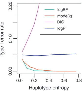
Results for inferred haplotypes:The power and type I error rates were calculated using the significance thresholds calculated for knownX. Figure 3 shows the mean type I error rates averaged overf, as a function of relative entropyH¯.
The logP had the correct error rate independent ofH¯, but at the nominal 5% significance level mode(k) was increasingly conservative asH¯ increases. The logBF statistic was also conservative, whereas the DICdiff
sta-tistic was extremely anticonservative (seeFile S1andFile S2for details of logBF and DICdiff). Hence mode(k) was
the preferred Bayesian statistic on the basis of perfor-mance and interpretation. It is also directly available as a model parameter with a posterior distribution.
The effect of the entropy,H¯on mode(k) is due to the Bayesian method properly taking into account the un-certainty in individuals’ haplotype assignments. Which-ever ‘‘true’’ haplotypes were selected to simulate the phenotype, the proportion of correct draws from the posterior will inevitably be lower at high entropy loci. Incorrect draws lead to incorrect parameter estimates, such that the individual haplotype estimates are closer to the overall mean than their true values, leading to shrinkage ink.
The weighted regression used for the F test does not properly allow for the haplotype uncertainty, but simply uses the expectations of individuals’ haplotype effects,pnT, which is difficult to interpret in terms of
haplotype pairs. If all haplotype pairs have very similar probabilities with only very small differences between them, the Bayesian model will have much less informa-tion and lower power whereas theFtest will be relatively unaffected. However, in the weighted regression, when the haplotype pair probabilities are almost equal (as when there is high entropy in the haplotype
assign-ments), this results in the least-squares estimatesTkˆ being unstable and taking very large nonsensical values.
In contrast, the Bayesian approach prevents this oc-curring by restricting the parameter values to the support Figure1.—Power to detect a QTL when
hap-lotypes are known, as a function of the QTL effect size as a percentage of the total phenotypic variance. Results are presented for a range of QTL allele frequencies, f ¼ the number of founder accessions out of 19, for the nominal 5% (A–D) and genomewide 0.08% (E–H) signif-icance thresholds. The statistics are mode(k) (red) and logP (blue).
Figure2.—MSE of estimates of individual haplotype pair
effects. (A) Comparison of histograms of MSEQTLfor
regres-sion (blue) and Bayesian (red) estimates, with (B) compari-son of MSEQTL between methods for each simulated data
of the posterior distributions. The Bayesian estimates of
Tk are shrunk consistently and predictably as the un-certainty in the haplotypes increases. This is demon-strated in Figure 4, by the relationship between MSEQTL
and MSEnull for the Bayesian estimates as entropy
in-creases, which indicates that the estimates are being shrunk toward the null model as the level of information in the genetic data falls. The corresponding plots for the regression estimates show no such relationship.
The relative type I error rates of the statistics were reflected in their power levels (Figure 5). For low locus entropy, they have similar power, as observed when the haplotype pairs are known or observed. The logP had the highest power for high entropy levels, due to the fact that it does not properly take into account the
uncer-tainty in the haplotypes. If the significance thresholds for both statistics are adjusted with increasing entropy to maintain the size of the test (i.e., fix the proportion of false positives), the power of mode(k) matches the power of logP and even exceeds it for small QTL effect sizes.
Real data analysis of Arabidopsis QTL: We illustrate the relative performance of logP and mode(k) with analysis of QTL in a population of A. thalianaMAGIC lines (Koveret al.2009). We analyzed two phenotypes,
days to germination and days to bolting time (Figures 6 and 7). (Bolting time was calculated as the number of days between germination and noting the first flower bud.)
At the genomewide threshold, there were one QTL for days to germination and three significant QTL for days to bolting time, with both statistics identifying the same QTL at this threshold. The Bayesian statistic, mode(k), has much less background noise across the genome than logP and additionally has the advantage of indicating the size of the effect of the QTL.
There is some population structure in the MAGIC lines, which potentially violates the assumptions of in-dependence in both Bayesian and frequentist analyses. Certain lines have ‘‘cousins’’ that share 25% of the genome by descent. This could lead to long-range link-age disequilibrium (LD) across chromosomes and ‘‘ghost’’ peaks in the association analysis. However, the LD patterns observed in the data show little sign of this phenomenon (Koveret al.2009). To confirm this, we
reran our analysis on the data with cousin lines removed and the results were unchanged (Figure S8andFigure S9inFile S2).
DISCUSSION
Our Bayesian single-locus hierarchical random-effects model has a complete factorization of the joint posterior distribution so does not require a costly MCMC step. Figure3.—Type I error rates when haplotypes are inferred,
as a function of the sample-average entropy at a locus for the 5% significance threshold. Locus error rates were calculated from 1000 simulated data sets at each locus. The statistics are mode(k) (red), logBF (light blue), DICdiff(pink), and logP
(dark blue).
Figure4.—Effect of
hap-lotype uncertainty on indi-vidual effect estimates, from the regression and Bayesian analyses in relation to the simulated values for the QTL model (MSEQTL) and
the null model (MSEnull).
(A) MSEQTL of regression
estimates; (B) MSEnull of
regression estimates; (C) MSEQTL of Bayesian
esti-mates; (D) MSEnullof
This gives it comparable analysis times to the frequentist ANOVA analysis. We extended the factorization to allow for uncertainty in inferred haplotypes, using a version of multiple imputation. This extension provides an exact solution that fully takes into account the degree of uncertainty in the haplotypes. When haplotypes are known, the analysis of 1000 loci and 500 subjects runs in
,2 min, and when haplotypes are inferred, the same analysis runs in,20 min. The increased running time is due to the calculation of the posterior distribution ofk, for each draw of haplotypes in the inferred haplotype model.
When the haplotype data are known, Bayesian and frequentist methods had virtually identical power, but the frequentist estimates of the haplotype effects were much less accurate than the Bayesian estimates. The
Bayesian model had lower power for QTL whose alleles were carried on haplotypes observed at low frequency, but this was due to the choice of prior for the haplotype pair effects. Altering the prior to estimate the haplotype pair frequencies from the data might fix this problem.
When the haplotypes are inferred, the null distribu-tions of several Bayesian summary statistics were af-fected, in different ways, by the degree of uncertainty in the haplotype assignments at a locus, leading to differ-ent type I error rates at differdiffer-ent loci in the genome. We find that the higher accuracy of the individual haplotype pair effect estimates from the Bayesian model remains for the inferred haplotype data, although the estimates from both methods are affected by the un-certainty in haplotype assignment. Moreover, the error in the Bayesian estimates was easily explained by the loss Figure5.—Power to detect a QTL for inferred
haplotypes for constant and adjusted thresholds, as a function of the sample-average entropy at a locus. Results are presented for a range of QTL effect sizes as a percentage of the total pheno-typic variance, for the nominal 5% (A–E) and ge-nomewide 0.08% (F–J) significance levels. Power is reported for the statistics mode(k) and logP for both constant thresholds [red, mode(k); blue, logP] and adjusted thresholds [pink, mod-e(k); light blue, logP].
Figure6.—Real data analysis of the
of information, with effect estimates shrunk toward the null model as the uncertainty increased, whereas the regression estimates became increasingly unpredictable and unreliable. Because the Bayesian method is more accurate than the frequentist even when haplotypes are known, this shows that the difference will persist whatever frequentist method is used to deal with haplotype un-certainty,e.g., EM instead of the regression method used here.
Our preferred Bayesian summary statistic is k, the proportion of variance due to the locus, as estimated by the mode of the posterior distribution. In addition to its natural interpretation as the effect size of the QTL,kis technically superior to the other Bayesian statistics we considered. First, it is less conservative than the approx-imate Bayes factor. Second, the DIC statistic is highly anticonservative and hence invalid at the 5% level. This is due to the use of plug-in likelihoods with the multiple imputation approach, which do not properly take into account the uncertainty in the haplotype inference, in contrast tok.
The F test also ignores uncertainty in the inferred haplotypes (as measured by the entropy) and conse-quently has much greater error in the estimation of the haplotype pair effects, although higher power at loci with higher entropy. The advantage of theFtest is that it has a well-defined constant significance threshold for any given size of test. The mode ofk-statistic loses power relative to theFtest as entropy increases, when a constant significance threshold is applied, because the type I error rate decreases. However, if the significance thresh-old for the mode of k-statistic is adjusted as entropy increases to maintain the type I error rate, it matches the power of theFtest and even exceeds it for small QTL effect sizes. Also, despite the effect of entropy on the null distribution, we found that the Bayesian model detected
the same QTL at the genomewide significance level, even when not adjusted, when analyzing a real data set. This emphasizes the importance of high-quality meth-ods for inferring haplotypes, such that the majority of loci in the genome have low levels of haplotype entropy. Our model can be extended to fit all loci simulta-neously, with a flat Dirichlet prior distribution for the loci proportions of variance. The Dirichlet distribution imposes natural constraints on the variance parameters, as the Uniform[0, 1] prior on the locus proportion of variance does for the single-locus model. Indeed, forcing the sum of the variances for all loci to not exceed the total phenotypic variance may act as a shrinkage prior without the need for an additional level of the hierarchical model. However, the single-locus analog of the Dirichlet distribution is the Beta distribution and our model is sensitive to the choice of parameters for a Beta prior. Hence it may be necessary to include these hyperparameters as unknowns in the model with flat hyperpriors, as described by Yi and Xu (2008). The
multilocus model would require MCMC techniques to sample from the joint posterior, similarly to the conven-tional model in Chapter 15 of Gelman et al. (2004).
Further research is needed into the added value of the multilocus model over our single-locus model for inferred genetic data to justify the additional computing time it would require.
LITERATURE CITED
Bardel, C., P. Darluand E. Genin, 2006 Clustering of haplotypes based on phylogeny: How good a strategy for association testing? Eur. J. Hum. Genet.14:202–206.
Durrant, C., K. T. Zondervan, L. R. Cardon, S. Hunt, P. Deloukas
et al., 2004 Linkage disequilibrium mapping via cladistic analy-sis of single-nucleotide polymorphism haplotypes. Am. J. Hum. Genet.75:35–43.
Figure7.—Real data analysis of the
Excoffier, L., and M. Slatkin, 1995 Maximum-likelihood estima-tion of molecular haplotype frequencies in a diploid populaestima-tion. Mol. Biol. Evol.12(5): 921–927.
Gelman, A., J. B. Carlin, H. S. Stern and D. B. Rubin, 2004 Bayesian Data Analysis, Ed. 2 (Texts in Statistical Science). Chapman & Hall/CRC, London/New York/Washington, D.C./ Boca Raton, FL.
Haley, C. S., and S. A. Knott, 1992 A simple regression method for mapping quantitative trait loci in line crosses using flanking markers. Heredity69:315–324.
Hawley, M. E., and K. K. Kidd, 1995 Haplo: A program using the em algorithm to estimate the frequencies of multi-site haplo-types. J. Hered.86(5): 409–411.
Igo, Jr., R. P., D. Londono, K. Miller, A. R. Parrado, S. R. E. Quade
et al., 2007 Density-based clustering in haplotype analysis for as-sociation mapping. BMC Proc.1(Suppl. 1): S27.
Jasra, A., C. C. Holmesand D. A. Stephens, 2005 Markov chain Monte Carlo methods and the label switching problem in Bayes-ian mixture modeling. Stat. Sci.20(1): 50–67.
Knight, J., D. Curtisand P. C. Sham, 2008 Clumphap: A simple tool for performing haplotype-based association analysis. Genet. Epidemiol.32:539–545.
Kover, P. X., W. Valdar, J. Trakalo, N. Scarcelli, I. M. Ehrenreichet al., 2009 A multiparent advanced generation in-ter-cross to fine-map quantitative traits in Arabidopsis thaliana. PLoS Genet.5(7): e1000551.
Li, N., and M. Stephens, 2003 Modelling linkage disequilibrium, and identifying recombination hotspots using SNP data. Genet-ics165(4): 2213–2233.
Lin, D. Y., and D. Zeng, 2006 Likelihood-based inference on haplo-type effects in genetic association studies. J. Am. Stat. Assoc. 101(473): 89–118.
Lin, D. Y., D. Zengand R. Millikan, 2005 Maximum likelihood es-timation of haplotype effects and haplotype-environment inter-actions in association studies. Genet. Epidemiol.29:299–312. Lin, D. Y., Y. Huand B. E. Huang, 2008 Simple and efficient analysis
of disease association with missing genotype data. Am. J. Hum. Genet.82:444–452.
Liu, J., C. Papasianand H.-W. Deng, 2007 Incorporating single-lo-cus tests into haplotype cladistic analysis in case-control studies. PLoS Genet.3(3): e46.
Long, J. C., R. C. Williamsand M. Urbanek, 1995 An e-m algo-rithm and testing strategy for multiple-locus haplotypes. Am. J. Hum. Genet.56:799–810.
Meuwissen, T. H. E., B. J. Hayesand M. E. Goddard, 2001 Prediction of total genetic value using genome-wide dense marker maps. Ge-netics157:1819–1829.
Molitor, J., P. Marjoramand D. Thomas, 2003 Fine-scale map-ping of disease genes with multiple mutations via spatial cluster-ing techniques. Am. J. Hum. Genet.73:1368–1384.
Morris, A. P., 2006 A flexible Bayesian framework for modeling haplotype association with disease, allowing for dominance
ef-fects of the underlying causative variants. Am. J. Hum. Genet. 79:679–694.
Mott, R., C. J. Talbot, M. G. Turri, A. C. Collinsand J. Flint, 2000 A method for fine mapping quantitative trait loci in outbred animal stocks. Proc. Natl. Acad. Sci. USA97(23): 12649–12654.
Park, T., and G. Casella, 2008 The Bayesian lasso. J. Am. Stat. As-soc.103(482): 681–686.
Qin, Z. S., T. Niuand J. S. Liu, 2002 Partition-ligation-expectation-maximization algorithm for haplotype inference with single-nu-cleotide polymorphisms. Am. J. Hum. Genet.71:1242–1247. Raftery, A. E., 1986 Choosing models for cross-classifications. Am.
Sociol. Rev.51(1): 145–146.
Sen, S´., and G. A. Churchill, 2001 A statistical framework for quan-titative trait mapping. Genetics159:371–387.
Spiegelhalter, D. J., N. G. Best, B. P. Carlinand A.van derLinde, 2002 Bayesian measures of model complexity and fit. J. R. Stat. Soc. Ser. B64(4): 583–639.
Stephens, M., and P. Donnelly, 2003 A comparison of Bayesian methods for haplotype reconstruction from population genotype data. Am. J. Hum. Genet.73(5): 1162–1169.
Stephens, M., N. Smithand P. Donnelly, 2001 A new statistical method for haplotype reconstruction from population data. Am. J. Hum. Genet.68:978–989.
Tachmazidou, I., C. J. Verzilliand M. D. Iorio, 2007 Genetic as-sociation mapping via evolution-based clustering of haplotypes. PLoS Genet.3(7): e111.
Threadgill, D. W., K. W. Hunterand R. W. Williams, 2002 Genetic dissection of complex and quantitative traits: from fantasy to real-ity via a communreal-ity effort. Mamm. Genome13:175–178. Tzeng, J.-Y., C.-H. Wang, J.-T. Kaoand C. K. Hsiao, 2006
Regression-based association analysis with clustered haplotypes through use of genotypes. Am. J. Hum. Genet.78:231–242.
Waldron, E. R. B., J. C. Whittakerand D. J. Balding, 2006 Fine mapping of disease genes via haplotype clustering. Genet. Epide-miol.30:170–179.
Wang, H., Y.-M. Zhang, X. Li, G. L. Masinde, S. Mohan et al., 2005 Bayesian shrinkage estimation of quantitative trait loci pa-rameters. Genetics170:465–480.
Xu, S., 2003 Estimating polygenic effects using markers of the entire genome. Genetics163:789–801.
Yi, N., and D. Shriner, 2008 Advances in Bayesian multiple quanti-tative trait loci mapping in experimental crosses. Heredity100: 240–252.
Yi, N., and S. Xu, 2008 Bayesian lasso for quantitative trait loci map-ping. Genetics179:1045–1055.
Zeng, D., D. Y. Lin, C. L. Avery, K. E. Northand M. S. Bray, 2006 Efficient semiparametric estimation of haplotype-disease associations in case-cohort and nested case-control studies. Bio-statistics7(3): 486–502.
Communicating editor: H. Zhao
APPENDIX: FACTORIZATION OF THE JOINT POSTERIOR
LetNbe the number of individuals in the sample and letKbe the number of genotypes at the genetic locus such that fork¼1,. . .,K, there areNkindividuals with genotypek, where theNkare observed (fixed) such thatPKk¼1Nk¼N. Let mbe the overall mean of the observed phenotypey, lets2be the total phenotypic variance, and letkbe the proportion
of the total phenotypic variance attributable to the genetic locus. LetTkbe the effect on the phenotype of genotypek. LetT¼[T1,. . .,TK]Tand letL(y,m,T,s2,k,X) be the likelihood function of the data and the parameters. Then using
Bayes’ rule, the (unnormalized) joint posterior distribution of all the parameters given the data is proportional to the likelihood multiplied by the priors, such that
pðm;T;s2;kjy;XÞ
}kK=2ð1kÞN=2sNK2exp 1 2s2
XK
k¼1
Tk2 k 1
1 ð1kÞ
XNk
i¼1
ðykimTkÞ2
" #
( )
Inspection of the joint posterior reveals that the posterior distribution ofTdepends on all of the other parameters,
m,s2,kand also that conditional on these parameters, the posterior distributions of theTk’s do not depend on each
other. Hence we first consider the conditional distribution ofTk, where
pðTjm;s2;k;y;XÞ ¼Y
K
k¼1
pðTkjm;s2;k;y;XÞ:
Conditional posterior distribution ofTk:To start the factorization we can write
pðT;m;s2;kjy;XÞ ¼ Y
K
k¼1
pðTkjm;s2;k;y;XÞ
" #
pðm;s2;kjy;XÞ; ðA2Þ
wherep(m,s2,kjy,X) does not depend onT. Hence pðTkjm;s2;k;y;XÞ}pðT;m;s2;kjy;XÞ
}exp 1
2s2 Tk2
k 1
1 ð1kÞ
XNk
i¼1
ðTk22ðykimÞTkÞ
" #
( )
¼exp 1 2s2
Tk2 k 1
Nk
ð1kÞT 2
k 2Tk
1 ð1kÞ
XNk
i¼1
ðykimÞ
" #
( )
¼exp Nk 2kð1kÞlks2
½Tk22TkðklkðykmÞÞ
;
whereyi¼ ð1=NiÞPNi
k¼1yikandlk¼1=ðk1ð1kÞ=NkÞ. This is the standard form of a normal distribution, so Tkjm;s2;k;y;X N klkðykmÞ;
klkð1kÞs2 Nk
;k¼1;. . .;K:
To continue the factorization in (A2), we must findp(m,s2,kjy,X) by integrating outTk,k¼1,. . .,Kfrom the joint
posterior (A1):
pðm;s2;kjy; XÞ ¼
ð . . .
ð
pðT;m;s2;kjy;XÞdT1 . . . dTK
}kK=2ð1kÞN=2sNK2Y
K
k¼1
ð
exp 1 2s2
Tk2 k 1
1 ð1kÞ
XNk
i¼1
ðykimTkÞ2
" #
( )
dTk
¼kK=2ð1kÞN=2sNK2Y
K
k¼1
exp 1
2s2ð1kÞ
XNk
i¼1
ðykimÞ2
( )
Y
K
k¼1
ð
exp Nk 2klkð1kÞs2½T
2
k 2TkðklkðykmÞÞ
dTk:
By comparison with the probability density function (pdf) of a normal distribution, adding and subtracting the extra term required to complete the square,
ð
exp Nk 2klkð1kÞs2½T
2
k 2TkðklkðykmÞÞ
dTk
} exp klkNkðykmÞ2
2ð1kÞs2
s kð1kÞ
ð1k1kNkÞ
1=2
}exp klkNkðykmÞ 2
2ð1kÞs2
s kð1kÞlk Nk
1=2 :
pðm;s2;kjy;XÞ
}kK=2ð1kÞN=2sNK2exp 1 2ð1kÞs2
XK
k¼1
XNk
i¼1
ðykimÞ2klkNkðykmÞ2
" #
( )
Y
K
k¼1
sðkð1kÞlkÞ1=2
¼ ð1kÞðKNÞ=2sN2 Y
K
k¼1
l1k=2
!
exp 1 2ð1kÞs2
XK
k¼1
XNk
i¼1
ðykimÞ2klkNkðykmÞ2
" #
( )
:
Conditional posterior distribution of mgiven s2,k:We have
pðm;s2;kjy;XÞ ¼pðmjs2;k;y;XÞpðs2;kjy;XÞ; ðA3Þ
wherep(s2,kjy,X) does not depend onm. Hence
pðmjs2;k;y;XÞ
}pðm;s2;kjy;XÞ
}exp 1
2ð1kÞs2
XK
k¼1
Nkðm22mykÞ½1klk
( )
¼exp 1 2ð1kÞs2 m
2X
K
k¼1
Nk
ð1kÞ ð1k1kNkÞ
2mX K
k¼1
Nkyk
ð1kÞ ð1k1kNkÞ
" #
( )
¼exp 1 2s2
XK
k¼1
lk
!
m22m
PK k¼1lkyk
PK k¼1lk
( )
:
This is the standard form of a normal distribution, so
mjs2;k;y;X N
PK k¼1lkyk
ðPK k¼1lkÞ
; s
2
ðPK k¼1lkÞ
:
To complete the expression in (A3), we must findp(s2,kjy,X) by integrating outmfrom the joint densityp(m,s2,kjy,X):
pðs2;kjy;XÞ ¼
ð
pðm;s2;kjy;XÞdm
}ð1kÞðKNÞ=2sN2 Y
K
k¼1
l1k=2
!
ð
exp 1
2ð1kÞs2
XK
k¼1
XNk
i¼1
ðykimÞ2klkNkðykmÞ2
" #
( )
dm
¼ ð1kÞðKNÞ=2sN2 Y
K
k¼1
l1k=2
!
exp 1
2ð1kÞs2
XK
k¼1
XNk
i¼1
y2kiklkNky2k
" #
( )
ð
exp 1 2s2
XK
k¼1
lk
!
m22m
PK k¼1lkyk
PK k¼1lk
( )
dm:
ð
exp 1 2s2
XK
k¼1
lk
!
m22m
PK k¼1lkyk
PK k¼1lk
( )
dm
¼exp 1 2s2
ðPK
k¼1lkykÞ2
ðPK k¼1lkÞ
ð
exp 1 2s2
XK
k¼1
lk
!
m
PK k¼1lkyk
PK k¼1lk
2
( )
dm
}s X
K
k¼1
lk
!1=2
exp 1 2s2
ðPK
k¼1lkykÞ2
ðPK k¼1lkÞ
:
Hence
pðs2;kjy;XÞ
}ð1kÞðKNÞ=2sN1 X
K
k¼1
lk
!1=2
YK
k¼1
l1k=2
!
exp 1 2ð1kÞs2
XN
n¼1
yn2kX K
k¼1
Nklkyk2 ð1kÞ
ðPK
k¼1lkykÞ2
ðPK k¼1lkÞ
" #
( )
:
Conditional posterior distribution ofs2given k:Write
pðs2;kjy;XÞ ¼pðs2jk;y;XÞpðkjy;XÞ; ðA4Þ wherep(kjy,X) does not depend ons2. Hence as before,
pðs2jk;y;XÞ
}pðs2;kjy;XÞ
}ðs2ÞððN21Þ11Þexp 1
2ð1kÞs2
XN
n¼1
y2nkX K
k¼1
Nklky2k ð1kÞ
ðPK
k¼1lkykÞ2
ðPK k¼1lkÞ
" #
( )
;
which is the standard form of a scaled inversex2-distribution,
s2jk;y;X Scaled Inverse-x2ðN 1;r2Þ; where
r2¼ 1
ðN 1Þð1kÞ
XN
n¼1
y2nkX K
k¼1
lky2k ð1kÞ
ðPK
k¼1lkykÞ2
ðPK k¼1lkÞ
" #
:
Posterior distribution ofk:To find an expression for the marginal posterior distribution ofk, we must integrate out
s2fromp(s2,kjy,X), pðkjy;XÞ
¼
ð
pðs2;kjy;XÞds2
}ð1kÞðKNÞ=2 X
K
k¼1
lk
!1=2
YK
k¼1
l1k=2
! ð
ðs2ÞððN1Þ=211Þ
exp ðN 1Þr 2
2s2
ds2
}ð1kÞðKNÞ=2 X
K
k¼1
lk
!1=2
YK
k¼1
l1k=2
!
ðrðN1ÞÞ
}ð1kÞðK1Þ=2 X
K
k¼1
lk
!1=2
YK
k¼1
l1k=2
!
X
N
n¼1
y2nkX K
k¼1
Nklky2k ð1kÞ
ðPK
k¼1lkykÞ2
ðPK k¼1lkÞ
fork2[0, 1]. This distribution is not of standard form, but it is continuous inkwith no singularities in the interval (0, 1). Atk¼1 the density is zero, while atk¼0,lk¼Nkand the density
pðk¼0jy;XÞ}N1=2 Y K
k¼1
Nk1=2
! XN
n¼1
y2nð
PK
k¼1NkykÞ2 N
" #ðN1Þ=2
is finite. Hence the posterior is proper.
Combining the results in (A1), (A2), and (A3), a factorization exists of the joint posterior distribution such that
pðm;T;s2;kjy;XÞ ¼ Y
K
k¼1
pðTkjm;s2;k;y;XÞ
" #
Supporting Information
http://www.genetics.org/cgi/content/full/genetics.109.113183/DC1
Bayesian Quantitative Trait Locus Mapping
Using Inferred Haplotypes
Caroline Durrant and Richard Mott
Copyright © 2010 by the Genetics Society of America
C. Durrant and R. Mott 2 SI
FILE S1
SUPPLEMENTARY METHODS:THE INFORMATION CRITERION BASED STATISTICS
The Log10 Bayes factor
The Bayes factor is used for comparing a discrete set of models. However, for the problem of testing a random effect, the
two models we compare are the null model, with all groups pooled (κ = 0) and the QTL model, with a random-effect
parameter for every haplotype pair, where κ indexes a continuous family of models. In this case the Bayes factor has been
shown to be highly sensitive to the number of groups in the data and also to the variance κσ2 of the group means in the prior
[Gelman et al 2004]. Hence we approximate the true Bayes factor by focusing on κ rather than the individual effects Tk.
There is a well-known approximation to the Bayes factor which can be calculated using the Bayesian Information Criterion
(BIC) [Raftery 1986], such that, in our situation, BFapprox = exp{-( BICnull - BICQTL )/2}, where BICnull = -2 log Lnull ( y |
µnull*, (σ2)null*, X ) + 2 log( N ), BICQTL = -2 log L( y | T*, µ*, (σ2)*, κ*, X ) + ( K + 3 )log( N ), and K is the number of
haplotype pair effect parameters T. Bayes factors greater than 1 favour the QTL model over the null model. T*, µ*, (σ2)*
and κ* are posterior point estimates of the model parameters, such as means or modes.
The BIC is known to suffer from a loss of power when there are many parameters in the model, due to an overly severe
penalty function. Since it is likely for multi-allelic loci that the number of haplotype pairs K will be large enough to affect the
power, we wish to focus on the locus proportion of variance parameter κ. In terms of deciding whether or not a given
genetic locus affects the phenotype it is κ which is of most interest, rather than the individual effect parameters T. Therefore
we calculate a modified form of the BIC, following the method for calculating the true Bayes factor, and use this modified
form to calculate the approximate Bayes factor. We calculate a ‘marginal likelihood' by integrating the likelihood of the data
over T with respect to their Bayesian priors:
Lmarg = ∫…∫ L( y | T, µ, σ2, κ, X) [ ∏k=1K( 2πκσ2 )^{-1/2} exp{-Tk2/2κσ2} ] dT1… dTK.
Then the BIC for the QTL model becomes BICQTL = -2 log Lmarg ( y | µQTL*, (σ2)QTL*, κ*, X ) + 3 log( N ), now apparently
with only three model parameters. (The null model BIC remains unchanged.)
The difference in DIC
The expected predictive deviance [Akaike 1974] has been suggested as a criterion of model fit with best out-of-sample
predictive power and for normal models it can be approximately estimated by the Deviance Information Criterion (DIC)
[Gelman et al 2004, Spiegelhalter et al 2002]. Positive values of DICdiff = ( DICnull - DICQTL ) favour the QTL model. The
DIC is calculated as DIC = pD + D( T, µ, σ2, κ ) using the Deviance D( T, µ, σ2, κ ) = -2 log L( y| T, µ, σ2, κ ) and the
quantity pD = ( D( T, µ, σ2, κ ) – D( T*, µ*, (σ2)*, κ* ) ), where D is the average of the Deviance, taken over all draws from
the joint posterior distribution.
T*, µ*, (σ2)* and κ* are plug-in estimates of the parameters, which along with estimates xn*, n = 1, 2, …, N are required to
C. Durrant and R. Mott 3 SI
taken in choosing which estimates to use. The effect parameters T and the phenotypic mean µ have Normal posterior
distributions, which are symmetric, so the posterior sample means were used as T* and µ*. For κ* we used the estimate of
the posterior mode, as calculated above. The posterior distribution of σ2 is also asymmetric, so the posterior mode was used
as (σ2)*. The mode was estimated similarly to the mode of κ, but using a Gamma distribution instead of a Beta.
The form of the plug-in estimates xn*, n = 1, 2, …, N is unclear. However, a simple re-arrangement of the likelihood
expression avoids this problem. The full model likelihood L( y | T, µ, σ2, κ, X ) can be re-written as
∝ (1 - κ)N/2σ-N exp{ -1/( 2(1 - κ)σ2 ) [ ∑n=1N yn2 + ∑k=1K Nk ( µ + Tk )(µ + Tk – 2yk
• ) ]}.
Now, instead of needing plug-in estimates xn*, we need Nk* and yk•*, k=1, …, K. The yk• are averages of Normally
distributed random variables which are i.i.d. when X is known, so we assume that they also follow a Normal distribution with
unknown mean and variance. The Nk , k=1, …, K follow a Multinomial distribution, so each Nk has a marginal Binomial
distribution. Hence if the data sample has enough individuals to allow a large-sample approximation, the marginal
distribution of each Nk should follow a Normal distribution, which is symmetric. Hence the sample means of Nk , k = 1, 2,
…, K were used, where the average was taken over the haplotype pair probabilities pn , n = 1, 2, …, N. Given our
C. Durrant and R. Mott 4 SI
FILE S2
SUPPLEMENTARY RESULTS
Results for known haplotypes
The power of the two information criterion based statistics was virtually identical to that of the other two statistics (Figure
S1). Both logBF and DICdiff suffered from the same rare haplotype effect as described for mode(κ), logBF more than the
other two.
FIGURE S1.—Power of all four statistics when haplotypes are known, as a function of the QTL effect size, measured as the percentage of the total phenotypic variance. The four statistics are logBF (pink), mode(κ) (black), DICdiff (light blue) and the
log p-value of the F test (dark blue).
The accuracy of the haplotype effect estimates, as estimated by the mean squared error (MSE) from the simulated values,
was much better for the Bayesian model than for the regression. The MSEs of the regression estimates were independent of
QTL effect size and QTL allele frequency (Figure S2). The Bayesian MSEs were independent of QTL allele frequency,
except for the rare single haplotype effect, but increased slightly with increasing QTL effect size, levelling off for QTL
accounting for more than 6-7% of the phenotypic variance (Figure S3). Figures S2 and S3 show data from a marker interval
with very balanced counts of the different haplotypes and hence do not show the rare haplotype effect. The relationship
between the Bayesian MSEs and the QTL effect size reflects the bounding effect of the Bayesian prior. The haplotype effect
estimates are bounded and restricted to a range of sensible values near the true value. The QTL effect is naturally bounded
below at zero, so for small QTL effects, the effect estimates are more tightly restricted by this extra bound than the effects for
C. Durrant and R. Mott 5 SI
do not show this effect because the errors for small QTL are caused mostly by over-estimates rather than under-estimates.
The regression allows much larger errors in the estimates than the Bayesian model.
FIGURE S2. —Boxplots of mean squared errors (MSEs) of regression estimates of haplotype effects as a function of A. the effect of the QTL effect size, measured as the percentage of the phenotypic variance due to the QTL, for a QTL allele carried on four of the 19 haplotypes and B. the effect of the QTL allele frequency for a 4% QTL. (Note log scale of y axes.) The box (or box-and-whisker) plots show the spread of the distribution of points generated by the simulation for the different entropy levels. The box shows the central 50% of the distribution, between the 25% and 75% quartiles, with the middle bar representing the median or 50% quartile. The whiskers extend to the furthest data point which is no more than 1.5 times the length of the box away from the box. Data points further away are plotted individually.
box-and-C. Durrant and R. Mott 6 SI
whisker) plots show the spread of the distribution of points generated by the simulation for the different entropy levels. The box shows the central 50% of the distribution, between the 25% and 75% quartiles, with the middle bar representing the median or 50% quartile. The whiskers extend to the furthest data point which is no more than 1.5 times the length of the box away from the box. Data points further away are plotted individually.
Behaviour of logBF and DICdiff for inferred haplotypes
The power and type I error rates were calculated using the significance thresholds calculated when haplotypes are known.
At the nominal 5% significance level logBF was increasingly conservative as H increases. Also, DICdiff was extremely and
increasingly anti-conservative at the 5% level, which meant it was invalid as a test statistic. The effect of the entropy, H on
the distributions of the Bayesian statistics affected the likelihood-based statistics logBF and DICdiff in particular, through the
plug-in parameter and data estimates. Figure S4 shows the effect of increasing uncertainty in haplotype assignment on the
null distributions of the three Bayesian statistics and also of pDqtl, the dimensionality parameter of the QTL model DIC.
FIGURE S4.—Effect of increasing entropy in haplotype assignment on the null distribution of logBF (A, B), mode(κ) (C, D),
DICdiff (E, F) and the dimensionality parameter of the QTL model DIC, pDqtl (G, H). The box (or box-and-whisker) plots
show the spread of the distribution of points generated by the simulation for the different entropy levels. The box shows the central 50% of the distribution, between the 25% and 75% quartiles, with the middle bar representing the median or 50% quartile. The whiskers extend to the furthest data point which is no more than 1.5 times the length of the box away from the box. Data points further away are plotted individually.
The comparison of the null distributions of mode(κ) for known and inferred data shows the effect of properly taking into
C. Durrant and R. Mott 7 SI
simulate the phenotype, the proportion of correct draws will inevitably be lower at high entropy loci. Incorrect haplotype
inferences lead to incorrect parameter estimates, such that the individual haplotype estimates are closer to the overall mean
than their ‘true’ values, leading to shrinkage in the estimated proportion of the variance due to the locus, κ.
This also caused an increase in the values of DICdiff in the null distribution as entropy increased (Figure S4, F), via the
decrease in the dimensionality parameter pD (Figure S4, H). As entropy increases, the estimated number of distinct
parameters in the model decreases, under-penalizing the likelihood. This led to higher values of the likelihoods for the QTL
model, increasing DICdiff in favour of the QTL model. The mean of null distribution of the deviance was not affected by
entropy, although the variance did decrease as the locus entropy increased (data not shown). Hence the decrease in the mean
of the null distribution of pD was due to the plug-in likelihood, which was also affected by the plug-in estimates for the data,
in particular. This can be most clearly seen in the null distribution of logBF, the ratio of penalized plug-in likelihoods. LogBF
was affected by the fall in the plug-in estimates of mode(κ) as entropy increased but also by the change in the plug-in
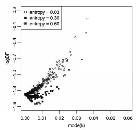
estimates of the group phenotype means yk . (Figure S5).
FIGURE S5.—Effect of increasing entropy in haplotype assignment on the relationship between logBF and mode(κ).
Figure S5 shows how the relationship between logBF and the effect size κ changed as the locus entropy increased. The
reduction in false positives for logBF as entropy increased was not simply because of the lower values of κ. An additional
effect was caused by the plug-in estimates of the phenotype means for the haplotype pair groups, which converged towards
the overall phenotype mean faster than the mode of κ decreased to zero as the locus entropy increased. The estimates of the
group phenotype means were also affected by properly taking into account the uncertainty in the haplotypes. The Bayesian
model accounts for this uncertainty in the estimate of κ, but the plug-in likelihood does not. Hence the type I error rate for
mode(κ) became less conservative than logBF as locus entropy increased. Figure S6 shows the power of logBF relative to
C. Durrant and R. Mott 8 SI
C. Durrant and R. Mott 9 SI
FIGURE S7.—Power when haplotypes are inferred, where the significance threshold was adjusted with increasing entropy to maintain the size of the test. Results are presented for a range of QTL effect sizes as a percentage of the total phenotypic variance, for the nominal 5% (A-E) and genome-wide 0.08% (F-J) significance thresholds. Power was calculated from 1,000 simulated data sets at each locus. The statistics are mode(κ) (red), logBF (light blue), DICdiff (green) and the log p-value of the
F test (dark blue).
Real Data Analysis without Cousin Lines
C. Durrant and R. Mott 10 SI
FIGURE S8.—Real data analysis of the phenotype Days to Germination, with cousin lines removed from the data set. Horizontal lines represent significance thresholds calculated via simulation: nominal 5% (dashed line) and genome-wide 0.08% (solid line). Vertical lines represent the boundaries between chromosomes.