Probe Design and Data Analysis for Gene Expression Microarrays

(1)

ABSTRACT

LILING WARREN. Probe Design and Data Analysis for Gene Expression Microarrays (Under the direction of Dr. Ben Liu)

This thesis work focuses on several bioinformatics aspects of DNA microarray experi-ments. DNA microarrays are breakthrough technologies for large scale gene expression profiling. Instead of measuring transcription levels one gene at a time, expression levels for many thousands of genes can be quantified simultaneously on one microarray. Depending on the array format, cDNA or pre-synthesized oligo nucleotides can be deposited as probes onto the array. Oligo probes can also be synthesized on the array. During the complete process of a DNA microarray experiment, many steps involve bioinformatics tasks; from probe design, image analysis, data normalization to data analysis and data mining. This thesis deals with oligo probe design issues and comparisons of data normalization methods. Methods on how to select a relatively small number of short probes and use them in a combinatorial fashion to quantify large scale expression levels are also explored.

(2)

linearly as the number of genes increases rather than exponentially. Detailed steps on how to implement the algorithm are outlined and examples are given. With some modifications, the algo-rithm can also be applied to design allele specific probes for SNP genotyping or point mutation detections.

In Chapter two, five normalization methods are compared with each other and also com-pared with analysis skipping the normalization step. Overall, performing normalization can reduce systematic variations and identify more genes as differentially expressed than without the normalization step. Among different normalization methods being compared, ANOVA based nor-malization method has the most power to detect differentially expressed genes. When the same normalization and analysis methods are used, ratio based method has more power than the one based on absolute signal intensity values. When different number of genes are detected by differ-ent normalization methods, one way to plan for future experimdiffer-ent is to use the set of genes that have been detected by all methods. Alternatively, one can use all the genes that have been identi-fied to be differentially expressed regardless which method was used to design further experi-ments. Insights from this study on how to incorporate biological variation into future experimental designs are also discussed.

(3)

(4)

Probe Design and Data Analysis for Gene

Expression Microarrays

by

Liling Warren

A dissertation submitted to the Graduate Faculty of North Carolina State University

in partial fulfillment of the requirements for the Degree of

Doctor of philosophy

BIOINFORMATICS RALEIGH

2002 APPROVED BY:

__________________________ __________________________ Ben H. Liu Bruce S. Weir

Chair of Advisory Committee

(5)

(6)

BIOGRAPHY

(7)

ACKNOWLEDGEMENTS

My sincere gratitude goes to my advisor, Dr. Ben Liu for his support, guidance and

encour-agement throughout my graduate study. Dr. Liu’s enthusiasm in biology, statistics and computer

science inspired me to enter the field of bioinformatics. He has provided direction for my

disserta-tion work and also helped me keep up with many exciting advancements in the areas of genomics

and bioinformatics. Bioinformatics is an integrated field that involves knowledge from many

intertwined disciplines and I truly thank Dr. Liu for his guidance and mentoring on helping me

learn things with both breadth and depth.

I would also like to express my great appreciation to my dissertation committee, Dr. Bruce Weir, Dr. Greg Gibson and Dr. Spencer Muse for their guidance, support and help on keeping me on the right track during my graduate research and studies.

I would like to thank my ex co-workers at the Center for Human Genetics, Duke University Medical Center. Having the experience of working in such a dynamic and productive group has kept me excited about front edge disease gene mapping research endeavors. Special thanks go to Dr. Eden Martin and Dr. Beth Hauser. It was such a pleasure to work with them and learn things from them.

(8)

have also helped me to stay focused on the real role of a bioinformatician - to apply statistics and computer theory and analysis tools to solve biological problems or testing biological hypothesis. I want to also express my many thanks to fellow graduate students in the Bioinformatics pro-gram and Ms. Amy Elkins for her wonderful assistance on getting things done.

(9)

LIST OF TABLES

Chapter 1

1. A list of microarray experiments . . . 29

2. A list of currently available microarray platforms . . . 29

3. A set of 13 yeast gene sequences . . . 30

4. Selected probes for the set of yeast genes . . . 31

5. SNPs and their flanking sequences . . . 32

6. Designed allele-specific probes for SNP genotyping . . . 33

Chapter 2 1. Summary of experimental results (Pritchard et al., 2001) . . . 60

2. The numbers of genes detected by different normalization methods with three different criteria: (1) Raw_P: no adjustment for multiple testing, using = 0.05; (2) Bonf_P: Bon-ferroni correction to ensure FWE (Family Wise Error rate = 0.05), using = 0.05/number of genes; (3) FDR_P: using False Discovery Rate, method of Benjamini and Hochberg (1995) to adjust for multiple testing. . . . 60

3. McNemar’s test comparison for a pair of methods . . . 61

(13)

from mcNemar’s tests. A value > 3.84 means the two methods are not equivalent. . 62 6. The numbers of genes detected by different smoothing parameters: numbers on the di-agonal are the numbers of genes detected with the specified smoothing option. Num-bers off the diagonal in the upper triangle are those that are detected by either or both of the two corresponding parameter specifications and the numbers off the diagonal in the lower triangle are the numbers of the genes that are commonly detected by both specifications . . . 62 Chapter 3

(14)

LIST OF FIGURES

Chapter 1

1. For a 41 mer where SNP site is located in the middle, there are 20 possible ways to select a 21 mer probe including the SNP site. . . . 28 2. The sequential order for constructing an all possible probe set for a 41 mer. Such ordering ensures that during the probe picking process, the probe that has the SNP site towards the middle is chosen when there are ties in terms of GC content or Tm value. . . . 28 Chapter 2

(15)

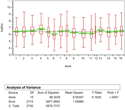
intensity values: box plot and ANOVA test show between block variation is highly

sig-nificant with a P value < 0.001. . . . 65

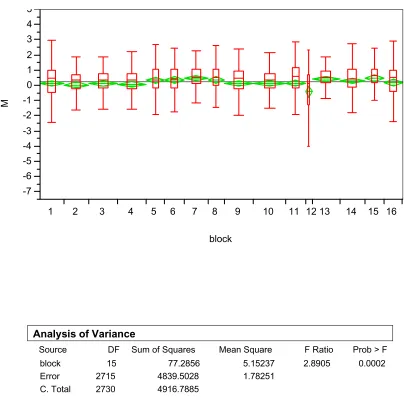
4. Assessing between block variation within kidney array 1 using log ratios: box plot and ANOVA test show between block variation is highly significant (P value = 0.0002). 66 5. Assessing dye effect within blocks 1 ~ 16 in kidney array 1: Scatter plots between M and A show the block specific dependence of M on A. (plots are ordered from top to bottom, left to right) . . . 67

6 (a). Loess adjustment for blocks 9-16 in kidney array 1: red points are original data, green point are predicted values from local smoothing fitting and blue points are residuals (plots are ordered from top to bottom, left to right) . . . 68

6 (b). Loess adjustment for blocks 9-16 in kidney array 1: red points are original data, green point are predicted values from local smoothing fitting and blue points are residuals (plots are ordered from top to bottom, left to right) . . . 69

7. F value histogram corresponding to method #1 . . . 70

(16)

16. P-values for genes that do not meet data quality criteria # 2 before and after using normalization method #1 . . . 74 17. Theoretical power curves for different numbers of replicates. Power curves from bottom to top: df2 = 12, 24, 36, 60, 120, corresponding to the number of replications = 2, 3, 4, 5, 10 respectively. . . . 75 18. Theoretical power curve for different numbers of mice and different numbers of replica-tions. For different color power curves from bottom to top: df2 = 12, 24, 36, 60, 120, cor-responding to the number of replications = 2, 3, 4, 5, 10 respectively. For different power curves with the same color, from bottom to top: df1 = 5, 10, 15, corresponding to the num-ber of mice = 6, 11 and 16 respectively . . . 76 19. 24 array means aross 6 mice in three tissues. From top to bottom: Testis, Kidney and Liv-er tissues. . . 77 Chapter 3

(17)

(18)

Chapter 1 A Novel Probe Design Algorithm

ABSTRACT

Motivation: DNA microarrays are tools to study expression profiles for many genes in parallel. For oligonucleotide-probe-based microarrays, choosing a set of gene-specific probes is a critical step to ensure reliable and accurate results. The set of probes deposited on the array share the same hybridization conditions during the experiment, thus it is important to design a set of probes that have the same or similar melting temperatures. With more genomes being fully sequenced and annotated, having an efficient and optimized probe design algorithm can be a very useful tool for oligo-based gene expression microarray experiments. When a differential hybridization approach is used for SNP genotyping, it is also desirable for all the allele-specific probes to have the same or similar melting temperatures.

(19)

opti-mized probe set. Users can input genes from a specific tissue, or a specific application to design probes for a microarray experiment. The probes can be either gene-specific or exon-specific, to allow for the study of alternative splicing. The algorithm can also be applied to design allele-spe-cific probes for SNP genotyping or mutation detection assays. We will use two examples to dem-onstrate how the algorithm works. The first example uses a set of yeast genes and shows how to design a gene-specific probe set for an expression microarray. The second example uses a set of SNPs within and around the APOE gene to show how to design allele-specific probes for SNP genotyping. Several variations to optimize the algorithm for different applications will be dis-cussed.

INTRODUCTION

With the ability to perform large numbers of hybridization reactions simultaneously, DNA

microarrays have shown great promise in genome-wide transcription profiling experiments, such

as identifying disease causing genes, identifying potential drug targets and classifying cancer

types. (Zhang et al., 1997; Golub et al. 1999; Perou et al., 2000) (Table 1). Depending on the

for-mat of the microarray, probes deposited on the chip can either be cDNA or oligonucleotides.

Oli-gonucleotide probes can also be synthesized on the chip (Table 2). There have been studies

suggesting that long oligo probes around 50~70 bases long are comparable to cDNA probes for

gene expression microarray experiments and have advantages in terms of cost reduction and data

accuracy (Kane et al., 2000). With more and more genomes being fully sequenced and annotated,

designing gene-specific or exon-specific oligonucleotide probes has become much more feasible.

(20)

microar-synthesized or deposited. In either case, probes are designed based on some proprietary algorithm

and users would not know how exactly they are chosen.

In this paper, we describe a novel algorithm for designing a set of high quality gene-specific

or exon-specific oligo probes that can share the same hybridization conditions for large scale

microarray experiments. It has been estimated that more than 60% of the genes have alternative

splicing at the transcript level (Lander et al., 2001; Venter et al., 2001), and being able to design

exon-specific probes can help users incorporate this important factor into their transcription

pro-filing studies. When designing probes for a gene expression study, the main criteria for a high

quality probe set should include:

(1) All of the probes have the same or similar melting temperatures. Melting temperature or Tm

is the temperature at which 50% of a given oligonucleotide is hybridized to its complementary

strand. It is a critical factor for hybridization based reactions.

(2) Probes are gene-specific, in order that cross hybridizations between genes and non-gene spe-cific probes can be avoided.

(3) Probes do not have major secondary structures such as internal loops, hairpins, bulged loops, etc. to inhibit efficient hybridizations between genes and probes.

(4) SNP variation sites in the probe sequence are avoided to increase the accuracy and specificity of the hybridization reactions. This criteria is less important for long probes than short probes.

(21)

Criteria (1) ~ (3) also apply to designing allele-specific probes for SNP genotyping. In addi-tion, the SNP variation site needs to be included, preferably towards the middle of the probe. To meet these criteria, the core algorithm is implemented to choose the best set of probes for a given set of sequences such that an optimized hybridization condition can be achieved. BLAST will be performed to ensure sequence specificity to avoid cross hybridization, and ZUKER will be incor-porated to avoid any significant secondary structure (Altschul et al., 1990; Lyngso et al., 1999).

ALGORITHM

When designing probes for microarray experiments, it is desirable for all of the probes to have similar lengths, and also to have melting temperatures similar enough that one common hybrid-ization condition is suitable for all hybridhybrid-ization reactions on the same microarray. Within each DNA sequence, there are many choices from which to pick a probe. Without an efficient algo-rithm, choosing a probe set out of all possible oligo combinations can be a daunting and computa-tionally demanding task. For instance, if there are m DNA sequences and n_i choices for sequence

i, there would then be probe combinations implying that equations need to be

eval-uated for selecting an optimal set of probes. For example, using a set of 500 DNA sequences with

a length of 1 kb on average, there are approximately 951500 possible 50 mer sets. As the number of DNA sequences increases, the number of computations increases exponentially. In this paper,

we show that an efficient algorithm may reduce this number of computations to , where c n_i

i=1

m

∏

n_i

i=1

m

∏

c n_i

i=1

m

(22)

(see Step Three). For the same example, the number of computations can be reduced to 50*500*591 for c = 50. As the number of sequences increases, this number only increases linearly rather than exponentially.

Design gene-specific or exon-specific probes for expression microarrays

The algorithm for designing gene-specific or exon-specific probes can be implemented in the following five steps.

Step One: For each DNA sequence, define a set of all subsequences of probe length. For exam-ple, for a DNA sequence that is bases long, there would be choices for selecting a

mer oligo as a probe. For each subsequence, a corresponding Tm can be calculated. Similarly, for

a set of m sequences, we can define the set of melting temperatures as ,

(1)

where each row denotes a sequence and elements within each row are the melting temperatures for all subsequences in that sequence. The numbers of elements in each of the rows (n₁, n₂, ..., n_m)

may or may not be the same, depending on the length of the sequence.

Step Two: Find the minimum and the maximum temperature values in the above melting temper-ature set, and .

L L–P+1 P

T

t₁₁ t₁₂ … t₁_n 1 t₂₁ t₂₂ … t₂_n

2

… … t_ij …

t_m₁ t_m₂ … t_mn

m

 

 

 

=

(23)

Step Three: Define a set of temperature values, , ,... ,... , between and with an

increment of , where c is the chosen number of incrementing steps between

and . In this paper, we will use rounded up integer values for melting temperatures in all

cal-culations and choose c to be the number of integers between and . Although it is

possi-ble to make the calculations more precise by keeping the decimal points, it is sufficient to treat

melting temperature values as integers for practical purposes. For each , find a probe set for all

sequences where each selected probe has the closest melting temperature to . For each , there

exists a vector of temperatures where each vector element is a melting temperature for the probe

of the choice from the corresponding sequence. We denote it as: = (t_k1, t_{k2 ...,}t_km).

Step Four: Calculate variance v_k for each of these as

. (2)

Step Five: Find the vector with the minimum variance . The oligo set corresponding to this

is the set of probes that has the most homogeneous melting temperatures for the given set of

gene sequences.

Calculate melting temperature

We have used two sets of formulae to calculate the melting temperature for each oligo. The t₁ t₂ t_k t_c t_min t_max

t_max–t_min

( )⁄c t_min

t_max

t_min t_max

t_k

t_k t_k

T_k

v_k

t_kl2

l=1

m

∑

t_kl

l=1

m

∑

 

 

 2

m

⁄

–

m–1

---=

T_k v_k

(24)

est neighbor (NN) thermodynamics approach (Borer et al., 1974) . For calculations based on sequence GC content, the following equation is used:

, (3)

where N is the total number of nucleotides in the sequence, and are the number of G’s and

C’s respectively (Wallace et al., 1979). The above equation assumes the standard conditions of 50nM for probe concentration and 50mM for salt concentration. When salt concentration needs to be adjusted, the following equation can be used:

T_m = 100.5 + 41 * (n_G+n_C) / N - 820 / N + 16.6 * log₁₀([Na+]), (4)

where 16.6*log₁₀([Na+]) is the term for adjusting salt concentration (Meinkoth et al., 1984).

When the NN thermodynamic approach is used, the melting temperature is computed as:

, (5)

where and are the enthalpy and entropy of the oligo. These two terms are computed with

the nearest neighbor schemes as and

respec-tively, where and are a pair of adjacent nucleotide bases. For example, for a putative

4mer CGAT that hybridizes with GCTA as:

(6) T_m= 64.9+41×(n_G+n_C–16.4)⁄N

n_G n_C

T_m ∆H

∆S+Rln(C_T⁄F)

---+16.6log₁₀([Na+])–273.15

=

∆H ∆S

∆H ∆H b( ,_ib_i₊₁)

i=1

n–1

∑

= ∆S ∆S b( ,_ib_i₊₁)

i=1

n–1

∑

=

b_i b_i₊₁ ∆H

∆H CGAT GCTA

 

 _{ ∆}_{H CG}

GC

 

 _{ ∆}_{H GA}

CT

 

 _{ ∆}_{H AT}

TA

   

+ +

(25)

and similarly, can be calculated as:

(7)

Besides and in Equation 5, R = 1.987 is the molar gas constant, and C_T

is the total oligonucleotide strand concentration. The value of F can be set to be 4 if the concentra-tion of the two strands being hybridized is similar or 2 if one strand is in excess (Borer et al., 1974; Breslauer et al., 1986).

Four sets of NN parameters for and are implemented in the program. Users have the

option to choose enthalpy and entropy parameter sets for DNA/DNA hybridizations proposed by Breslauer et al. (Breaslauer et al., 1986), SantaLucia (SantaLucia J.Jr., 1998), Sujimoto et al. (Sujimoto et al., 1995), or SantaLucia et al. (SantaLucia et al., 1996).

Design allele-specific probes for SNP genotyping

With some modifications, the algorithm can be applied to design allele-specific probes for SNP genotyping and point mutation detection. SNPs are Single Nucleotide Polymorphisms that occur roughly about every 1kb along human genomes (Lander et al., 2001). They can be powerful molecular markers for linkage and/or association disease gene mapping studies and pharmacoge-nomic applications. An international SNP consortium has been formed to make SNP's sequences and primers publicly available. Based on its latest, the tenth release of human SNPs, there have been nearly 1.5 million SNPs discovered and characterized in the human genome (Sachidanan-dam et al., 2001).

∆S

∆S CGAT GCTA

 

 _{ ∆}_{S CG}

GC

 

 _{ ∆}_{S GA}

CT

 

 _{ ∆}_{S AT}

TA

   

+ +

=

∆H ∆S cal⁄(°C⋅mol)

(26)

When the differential hybridization approach is used for SNP genotyping, allele-specific probes are first deposited or synthesized on the chip and labeled target DNAs are then applied onto the chip. Upon hybridization, captured fluorescent signals can be used to determine the pres-ence or abspres-ence of a certain allele. Besides having similar melting temperatures, probes being designed for SNP genotyping must include the SNP variation site, and have the variation site as close to the center of the probe as possible. Again, it is important to avoid cross hybridization and significant RNA secondary structure in the probe sequence, as in the case of designing probes for gene expression profiling. To ensure that a uniform condition can be applied to all of the hybrid-ization reactions, we try to choose probes with similar melting temperatures. For short oligos, the classical Tm = 2*(A+T) + 4*(G+C) calculation can be used (Wallace et al., 1979). Finding probes that have similar Tm is equivalent to choosing probes that have similar GC content. Here, GC content means the total number of G’s and C’s in a given DNA sequence. The following four steps describe how to find a set of allele-specific probes for SNP genotyping.

Step One: From the input DNA sequences flanking SNP sites, create a set of subsequences for each SNP variation. If the length of the probe is p, then the length of the subsequence is (2p-1) and the SNP site is located at the center position of the subsequence. For example, for a 41 mer as shown in Figure 1, the SNP site is located right in the middle, and there are 20 possibilities from which to choose a 21 mer probe for this variation. For each SNP, this step is done for both alleles.

(27)

, (8)

where each row denotes an oligo sequence, and elements within each row are the GC content val-ues for all possible probe choices in that oligo sequence.

Step Three: For 21 mer probes, the GC content can only take values from 0 to 21. For each GC value, we search through all possible probes for each SNP and find the one that is closest to the given GC value.

In doing the above step, there are two things we need to consider. One is that there are ties in terms of GC content when choosing the probe for a SNP allele. We want to choose the one that has the SNP variation site close to the center. To ensure this, we start out by putting the SNP vari-ation site in the center of the probe, then slide one window to the left and one to the right, one nucleotide at a time, as shown in Figure 2. When there are ties in terms of GC content, the oligo set constructing in this order ensures that the one that has the SNP site towards the center is picked first. The second thing we need to consider is that we try not to have SNP sites at the end of the probe. To balance this with minimizing GC content, we can set a range for the sliding win-dow and exclude cases where the SNP site is at the end of the probe.

Step Four: From step three, we have chosen the best set of the probes for each possible GC con-tent value. In this final step, we calculate the variance of GC concon-tent among probes for each

pos-GC

GC₁₁ GC₁₂ … GC₁_n 1 GC₂₁ GC₂₂ … GC₂_n

2

… … GC_ij …

GC_m₁ GC_m₂ … GC_mn

m

 

 

 

(28)

Optimizing other probe properties

During the process of implementing the core algorithm as described in the above section, we also need to check for probe quality such that the probe does not cross hybridize with other genes and also does not have unwanted major secondary structures. To accomplish such two tasks, we have incorporated two existing software programs, BLAST (Altschul et al., 1990) and ZUKER (Lyngso et al., 1999) into the main program. The executables of BLAST and ZUKER are called in the main program. The returned results are parsed to decide whether the probe is of good quality. If an oligo is rejected, the same probe picking process is repeated from step two until a good probe is found. The rejected oligo is excluded from the process.

BLAST is a widely used sequence alignment program that uses a heuristic algorithm for fast

local alignment. With BLAST, sequence similarity results are summarized by E values, where E

stands for Expectation. An E value represents the number of different alignments that have the

alignment scores equivalent to or better than the calculated one are expected to occur in a

data-base search by chance . A small E value indicates a significant search result. When a significant E

value is reported for the query sequence and a target sequence in the database, it means the

proba-bility that the sequence similarity shared by the two is caused by chance alone is highly unlikely.

Here, the ungapped BLAST was incorporated and an E value smaller than 0.05 is used as the cut

off value. A relatively relaxed sequence homology cut off value is chosen here to ensure high

sequence specificity for a given probe. Once a significant hit is found, another round of the probe

picking process is repeated until no more significant hits are found. Again, the rejected oligo is

(29)

The local stand alone BLAST program was downloaded from NCBI anonymous FTP server

(ftp://ftp.ncbi.nih.gov) under /blast/executables/. As required, the set of sequences being checked

against first needed to be formatted. When designing probes for gene expression applications,

probes need to be checked against the formatted genome mRNA pool sequences. For human,

mouse and rat applications, corresponding UniGene sequences can be used for such purposes

(Schuler, G.D., 1997). UniGene is a collection of expressed genes or EST (Expressed Sequence

Tag) sequences. It also has the information about in which tissue a gene or an EST is expressed.

For SNP genotyping and mutation detection, PCR is likely done before hybridization. It is thus

necessary only to blast probes against DNA sequences flanking SNPs being genotyped to ensure

probe specificity.

(30)

(9)

where s_i can be any of the RNA sub-structures such as stacked pairs, internal loops, etc (Zuker, et

al., 1999; Zuker, M., 1987).

ZUKER was downloaded from http://www.brics.dk/~rlyngsoe/zuker/. A free energy score for a given mRNA sequence can be parsed from its output. A relatively stringent cut off criteria (total energy score < 15 for 50mers, for example) is used to determine whether the probe sequence has any unwanted secondary structure. When the probe cannot pass this check, another round of the probe picking process is subsequently carried out until the probe sequences do not posses any major secondary structure. Both calling BLAST and calling ZUKER are done during the process and a probe is kept only when it passes both checks.

When SNP sites and conserved functional domain region(s) need to be avoided during probe designs for gene expression experiments, sites and regions that need to be avoided can be speci-fied as input to the program along with the DNA sequence information. The program can take such input and avoid choosing probes in those regions. Avoiding SNP sites is especially important for relatively short probes, where sequence non-specificity, caused by SNP variation in the probe sequence, can have a relatively larger impact on the hybridization efficiency than on longer probes.

E S( ) e s( )_i

i=1

m

∑

(31)

EXAMPLES

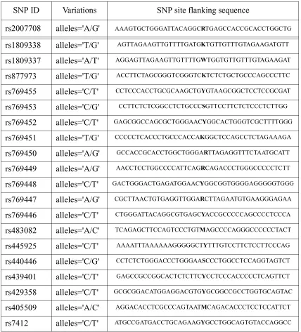
We use the following two examples to illustrate how the algorithm works. The first one shows how to design a set of 50 mers for 13 yeast genes as shown in Table 3. For illustration purposes, we selected a set of short genes in this example, so that the detailed steps of the algorithm can be shown. In the second example, we demonstrate how to apply the algorithm to design a set of allele-specific 21 mers to genotype 20 SNPs in a 8 kb region surrounding the APOE gene, a well recognized disease susceptibility gene for Alzherimer disease (Pericak-Vance et al., 1991). SNP flanking sequence information is downloaded from NCBI web site: http://www.ncbi.nlm.nih.gov/ SNP/ and the set of SNPs within and around the APOE gene are obtained from NCBI’s Refseq resource (Pruitt et al., 2001).

Example 1: Gene Expression Study

In the first example, we show how to design a set of 50 mer probes for 13 yeast genes listed in Table 3. We follow the same steps as described in the algorithm section.

(32)

, (10)

where each row corresponds to a gene and each element in the row is the melting temperature for a subsequence.

Step Two: Find the minimum and maximum melting temperature values in the above matrix. In this case, the minimum is 71 and the maximum is 111 (value not shown).

Step Three: For each temperature value within the range between minimum, 71, and maxi-mum, 111, find a vector of temperature values where each element in the vector corresponds to a

subsequence that has the closest melting temperature to . The starting position for each probe is

also recorded. For example, when = 71, the corresponding closest melting temperature vector

is: (71, 73, 88, 92, 87, 88, 94, 87, 95, 87, 94, 88, 93) and the corresponding starting position vector is: (0, 98, 76, 262, 42, 145, 19, 235, 120, 316, 176, 116, 253).

Step Four: Calculate the variance for each vector of the melting temperatures as described in step three. For melting temperatures (71, 72, 73, 74, 75, 76, 77, 78, 79, 80, 81, 82, 83, 84, 85, 86, 87, 88, 89, 90, 91, 92, 93, 94, 95, 96, 97, 98, 99, 100, 101, 102, 103, 104, 105, 106, 107, 108, 109,

T

71 71 72 72 73 73 … 104 104 91 92 91 92 93 92 … 74 74 91 92 90 89 89 91 … 92 92 103 104 103 103 103 103 … 103 103

95 95 94 94 94 94 … 107 107 96 97 96 95 96 97 … 99 100 96 97 96 96 95 96 … 98 98 101 103 102 101 101 101 … 92 91 101 102 101 101 101 102 … 96 95 99 99 98 98 98 96 … 91 91 98 99 99 98 97 95 … 97 95 90 91 89 89 89 89 … 96 96 96 96 96 96 96 96 … 100 98

(33)

110, 111), the corresponding variances are (214, 202, 190, 179, 168, 157, 146, 136, 124, 113, 102, 92, 80, 69, 58, 47, 36, 28, 23, 18, 13, 8, 4, 1, 0, 0, 1, 2, 3, 4, 5, 6, 7, 9, 13, 19, 27, 35, 45, 56, 68).

Step Five: For t_i’s between 71 and 111, find the one that has the smallest variance. In this case, the vector corresponding to = 96 and = 95 both have zero variances. This indicates there are two

probes sets that have homogeneous melting temperatures. Either set of probes can be final choice

for the 13 yeast genes. For = 96, the results are summarized in Table 4.

Example 2: SNP Genotyping

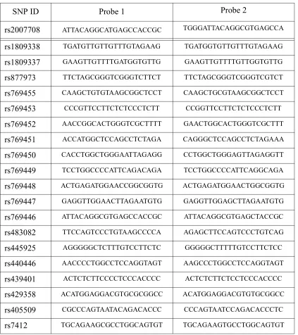
In the second example, we show how to implement the algorithm to design allele-specific probes for either SNP genotyping or point mutation detection applications. Table 5 lists 20 SNPs

within and around APOE gene and their flanking sequences. The goal is to design 21 mer probes to genotype the set of SNPs based on differential hybridization, i.e. to determine the presence or absence of a specific allele based on differences in two allele-specific hybridization results.

Step One: For each SNP, construct a set of 21 mers that include the SNP site somewhere in the sequence. For example, for SNP rs2007708, there are 20 possible choices that can be constructed as shown in Figure 1. The set of possible probes include: AGTGCTGGGATTACAGGCRT, GTGCTGGGATTACAGGCRTG, ..., CRTGAGCCACCGCACCTGGC, where R denotes an A/ G variation.

Step Two: Count the numbers of G’s and C’s in each possible probe and create a GC content set, where each row consists of counts of G’s and C’s within a possible probe as constructed in Step

t_i t_i

(34)

One. In this case, the first and second rows of the set would be (10, 11, ... , 14) and (11, 12, ... , 15), corresponding to the two alleles of the first SNP.

Step Three: For each GC value within the range of possible counts of G’s and C’s for 21 mers, i.e., any integer between 0 and 21, find a probe set where each probe has the closest GC value among all possible probe choices for a given SNP allele. In this case, when GC=5, the set of probes identified has a vector of GC values as ( 11, 12, 6, 7, 7, ... , 13, 12).

Step Four: Identify the GC value which has the smallest variation of GC count within the corre-sponding probe set. In this example, the smallest variance is 2.8 when GC=12 and the correspond-ing set of probes is listed in Table 6.

DISCUSSION

(35)

that have very different Tm range from the rest of the genes, choosing an optimized probe set using our algorithm would be highly influenced or restricted by the particular one or few genes. In such a situation, it is recommended to design the probe set first for all of the genes excluding one or few genes, then incorporate them later. It might be necessary to adjust the probe length for the genes incorporated last. These kinds of genes can be identified before running the probe design program. They are either very short or have many repeats in the sequence, resulting a narrow range of Tm for a given probe length.

When designing gene-specific or exon-specific probes, sometimes it is preferable to select a probe that is located at the 5’ end of the sequence. This can be easily achieved by starting the probe-choosing process from 5’ to 3’. Then the first one meeting the selection criteria will be located preferably more towards 5’ end. We can also use only a set of subsequences that start from the 5’ end of all the sequences for probe design. The results are thus guaranteed to be biased towards the 5’ end of the sequences.

When there are unknown nucleotide(s) in the possible probe sequence during the probe

pick-ing process, the correspondpick-ing is set to be an arbitrarily small number, much smaller than

other possible melting temperature values. By doing this, the probe set including this sequence would have a higher variance thus the chance for this probe set to be chosen is quite small. This helps to avoid chosen probes having unknown nucleotide(s)

Sometimes it is difficult to find a set of homogeneous probe set in terms of Tm or GC con-tent simply because one or few genes have a very different base composition compared to all

(36)

Besides designing probes for SNP genotyping, the same method can be applied to design probes for diagnostic chips, which can be used to screen many disease point mutations simulta-neously. Instead of host DNA, bacterial or virus DNA or RNA can also be put on the chip, allow-ing us to design chips to diagnose infectious diseases.

When applying the algorithm described here to design probes for SNP genotyping or point mutation identification, it is possible that a single optimized hybridization condition can not be found due to the fact that SNP site flanking sequence may have very different GC content. One way to solve this problem is to perform a different batch of hybridization reactions for different melting temperature groups.

In practice, the differential hybridization based SNP genotyping technique itself may not have great advantages in comparison with numerous other competing SNP genotyping techniques such as Pyrosequencing (Ronaghi, M., 2001) and the TaqMan assay (Holland et al., 1991). It is up to the researchers to decide which method to use by weighing various factors including overall cost, ease of following the protocol and data accuracy. When the differential hybridization method is the choice, the algorithm presented here can help find the best set of allele-specific probes for SNP genotyping.

CONCLUSIONS

(37)

BLAST and ZUKER are incorporated, the probe quality can be further improved and thus improve the accuracy of hybridization reaction based microarray experiments.

ACKNOWLEDGEMENT

We thank Dr. Yinghsuan Sun, Dr. Ross Whetten, Dr. Lun Xiao, and Mr. Jeff Soo Hoo for their helpful suggestions and comments.

REFERENCES

Altschul,S.F., Gish,W., Miller,W., Myers,E.W., Lipman,D.J. (1990) Basic local alignment search tool. J. Mol. Biol., 215, 403-410.

Bittner,M., Meltzer,P., Chen,Y., Jiang,Y., Seftor,E., Hendrix,M., Radmacher,M., Simon,R., Yakhini,Z., Ben-Dor,A., Sampas,N., Dougherty,E., Wang,E., Marincola,F., Gooden,C., Lued-ers, J., Glatfelter,A., Pollock,P., Carpten,J., GillandLued-ers,E., Leja,D., Dietrich,K., Beaudry,C., Berens, M., Alberts,D., Sondak,V. (2000) Molecular classification of cutaneous malignant melanoma by gene expression profiling. Nature, 406, 536-540.

Blanchard,A.P. (1998) Synthetic DNA Arrays. Genetic Engineering, 20, 111-123.

Blanchard,A.P. and Friend,S.H. (1999) Cheap DNA arrays-it's not all smoke and mirrors. Nat. Biotechnol., 17, 953.

(38)

Borer,P.N., Dengler,B., Tinoco,I.Jr., Uhlenbeck,O.C. (1974) Stability of ribonucleic acid double-stranded helices. J Mol Biol., 86(4), 843-853.

Chee,M.S., Yang,R., Hubbell,E., Berno,A., Huang,X.C., Stern,D., Winkler,J., Lockhart,D.J., Morris,M.S. and Fodor,S.P.A. (1996) Accessing Genetic Information with High-Density DNA Arrays. Science, 274, 610-614.

Davis,R.E., Staudt,L.M. (2002) Molecular diagnosis of lymphoid malignancies by gene expres-sion profiling. Curr Opin Hematol., 9, 333-338.

DeRisi,J.L., Iyer,V.R., Brown,P.O. (1997) Exploring the metabolic and genetic control of gene expression on a genomic scale. Science, 278, 680-686.

Edman,C.F., Raymond,D.E., Wu,D.J., Tu,E., Sosnowski,R.G., Butler,W.F., Nerenberg,M., Heller,M.J. (1997) Electric field directed nucleic acid hybridization on microchips. Nucleic Acids Res., 25, 4907-4914.

Fodor,S.P., Read,J.L., Pirrung,M.C., Stryer,L., Lu,A.T., Solas,D. (1991) Light-directed, spatially addressable parallel chemical synthesis. Science, 251, 767-773.

Golub,T.R., Slonim,D.K., Tamayo,P., Huard,C., Gaasenbeek,M., Mesirov,J.P., Coller,H., Loh, M.L., Downing,J.R., Caligiuri,M.A., Bloomfield,C.D., Lander,E.S. (1999) Molecular classifi-cation of cancer: class discovery and class prediction by gene expression monitoring. Science, 286, 531-537.

(39)

Heller MJ, Forster AH, Tu E. (2000) Active microeletronic chip devices which utilize controlled electrophoretic fields for multiplex DNA hybridization and other genomic applications. Elec-trophoresis, 21, 157-164.

Holland,P.M, Abramson,R.D, Watson,R., Gelfand,D.H. (1991) Detection of specific polymerase chain reaction product by utilizing the 5'----3' exonuclease activity of Thermus aquaticus DNA polymerase. Proc Natl Acad Sci., 88, 7276-80.

Hughes,T.R., Mao,M., Jones,A.R., Burchard,J., Marton,M.J., Shannon,K.W., Lefkowitz,S.M., Ziman,M., Schelter,J.M., Meyer,M.R., Kobayashi,S., Davis,C., Dai,H., He,Y.D., Stephaniants,S.B., Cavet,G., Walker,W.L., West,A., Coffey,E., Shoemaker,D.D., Stoughton, R., Blanchard,A.P., Friend,S.H. and Linsley,P.S. (2001) Expression profiling using microar-rays fabricated by an ink-jet oligonucleotide synthesizer. Nat Biotechnol., 19, 342-347.

Hughes,T.R., Marton,M.J., Jones,A.R., Roberts,C.J., Stoughton,R., Armour,C.D., Bennett, H.A., Coffey,E., Dai,H., He,Y.D., Kidd,M.J., King,A.M., Meyer,M.R., Slade,D., Lum,P.Y., Stepa-niants,S.B., Shoemaker,D.D., Gachotte,D., Chakraburtty,K., Simon,J., Bard,M. and Friend, S.H. (2000) Functional discovery via a compendium of expression profiles. Cell, 102, 109-126.

Kane,M.D., Jatkoe,T.A., Stumpf,C.R., Lu,J., Thomas,J.D., Madore,S.J. (2000) Assessment of the sensitivity and specificity of oligonucleotide (50mer) microarrays. Nucleic Acids Res., 28, 4552-4557.

(40)

Lander, E.S. et al. (2001) Initial sequencing and analysis of the human genome. Nature, 409, 860-921

Lee,C.K., Weindruch,R., Prolla,T.A. (2000) Gene-expression profile of the ageing brain in mice. Nat Genet., 25, 294-297.

Lipshutz,R.J., Fodor,S., Gingeras, T., and Lockhart, D. (1999) High-density synthetic oligonucle-otide arrays. Nat. Genet. 21 (Suppl.), 20-24.

Lyngso, R.D., Zuker, M. and Pedersen, C.N. (1999) Fast evaluation of internal loops in RNA sec-ondary structure prediction, Bioinformatics, 15, 440-445.

Meinkoth,J., and Wahl,G. (1984) Hybridization of nucleic acids immobilized on solid supports. Anal Biochem, 138, 267-284.

Pericak-Vance,M.A., Bebout,J.L., Gaskell,P.C., Yamaoka,L.A., Hung,W-Y., Alberts,M.J., Walker,A.P., Bartlett,R.J., Haynes,C.S., Welsh,K.A., Earl,N.L., Heyman,A., Clark,C.M., Roses,A.D. (1991) Linkage studies in familial Alzheimer's disease: Evidence for chromosome 19 linkage. Am J Hum Genet., 48, 1034-1050.

Perou,C.M., Sorlie,T., Eisen,M.B., van de Rijn,M., Jeffrey,S.S., Rees,C.A., Pollack,J.R., Ross, D.T., Johnsen,H., Akslen,L.A., Fluge,O., Pergamenschikov,A., Williams,C., Zhu,S.X., Lon-ning,P.E., Borresen-Dale,A.L., Brown,P.O. and Botstein, D. (2000) Molecular portraits of human breast tumours. Nature, 406, 747-752.

(41)

Ramakrishnan,R., Dorris,D., Lublinsky,A., Nguyen,A., Domanus,M., Prokhorova,A., Gieser,L., Touma,E., Lockner,R., Tata,M., Zhu,X., Patterson,M., Shippy,R., Sendera,T.J., Mazumder,A. (2002) An assessment of Motorola CodeLink microarray performance for gene expression profiling applications. Nucleic Acids Res., 30, e30.

Ronaghi,M. (2001) Pyrosequencing sheds light on DNA sequencing. Genome Res., 11, 3-11.

Sachidanandam,R., Weissman,D., Schmidt,S.C., Kakol,J.M., Stein,L.D., Marth,G., Sherry,S., Mullikin,J.C., Mortimore,B.J., Willey,D.L., Hunt,S.E., Cole,C.G., Coggill,P.C., Rice,C.M., Ning,Z., Rogers,J., Bentley,D.R., Kwok,P.Y., Mardis,E.R., Yeh,R.T., Schultz,B., Cook,L., Davenport,R., Dante,M., Fulton,L., Hillier,L., Waterston,R.H., McPherson,J.D., Gilman,B., Schaffner,S., Van Etten,W.J., Reich,D., Higgins,J., Daly,M.J., Blumenstiel,B., Baldwin,J., Stange-Thomann,N., Zody,M.C., Linton,L., Lander,E.S., Altshuler,D. (2001) A map of human genome sequence variation containing 1.42 million single nucleotide polymorphisms, Nature, 409, 928-33.

SantaLucia,J.Jr. (1998) A unified view of polymer, dumbbell, and oligonucleotide DNA nearest-neighbor thermodynamics. Proc. Natl Acad. Sci. U S A, 95, 1460-1465.

SantaLucia,J.Jr., Allawi,H.T., Seneviratne,P.A. (1996) Improved nearest-neighbor parameters for predicting DNA duplex stability. Biochemistry, 35, 3555-3562.

(42)

Sugimoto,N., Nakano,S., Yoneyama,M., Honda,K. (1996) Improved thermodynamic parameters and helix initiation factor to predict stability of DNA duplexes. Nucleic Acids Res., 24, 4501-4505.

Schuler,G.D. (1997) Pieces of the puzzle: expressed sequence tags and the catalog of human genes. J Mol Med., 75, 694-698

Sugimoto,N., Nakano,S., Katoh,M., Matsumura,A., Nakamuta,H., Ohmichi,T., Yoneyama,M., Sasaki,M. (1995) Thermodynamic parameters to predict stability of RNA/DNA hybrid duplexes. Biochemistry, 34, 11211-11216.

zuker: http://www.brics.dk/~rlyngsoe/zuker/

Venter, J.C. et al. (2001) The sequence of the human genome. Science, 291, 1304-1351.

Wallace,R.B., Shaffer,J., Murphy,R.F., Bonner,J., Hirose,T., and Itakura,K. (1979) Hybridization of synthetic oligodeoxyribonucleotides to phi chi 174 DNA: the effect of single base pair mis-match. Nucleic Acids Res., 6, 3543-3547

Walt,D.R. (2000) Techview: molecular biology. Bead-based fiber-optic arrays. Science, 287, 451-452.

Yeakley,J.M., Fan,J.B., Doucet,D., Luo,L., Wickham,E., Ye,Z., Chee,M.S., Fu,X.D. (2002) Profil-ing alternative splicProfil-ing on fiber-optic arrays. Nat Biotechnol., 20, 353-358.

Zhang,L. Zhou,W., Velculescu,V.E., Kern,S.E., Hruban,R.H., Hamilton,S.R., Vogelstein,B. and Kinzler,K.W. (1997) Gene expression profiles in normal and cancer cells. Science 276, 1268-1272.

(43)

(44)

(45)

3’ AAAGTGCTGGGATTACAGGCRTGAGCCACCGCACCTGGCTG 5’

... ... probe 1

probe 2 probe 3 probe 4 probe 5 ...

Figure 1. For a 41 mer where SNP site is located in the middle, there are 20 possible ways to select a 21 mer probe including the SNP site.

... probe 20

3’ AAAGTGCTGGGATTACAGGCRTGAGCCACCGCACCTGGCTG 5’

... probe 1

probe 2 probe 3 probe 4 probe 5

Figure 2. The sequential order for constructing an all possible probe set for a 41 mer. Such ordering ensures that during the probe picking process, the probe that has the SNP site towards the middle is chosen when there are ties in terms of GC content or Tm value.

... ... probe 20

(46)

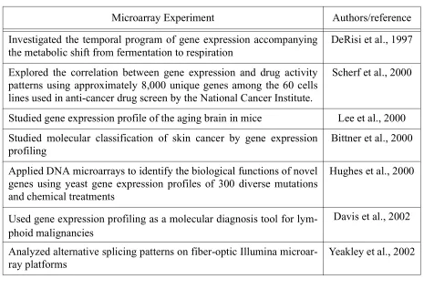
Table 1: A list of microarray experiments

Table 2: A list of currently available microarray platforms

Microarray Experiment Authors/reference

Investigated the temporal program of gene expression accompanying the metabolic shift from fermentation to respiration

DeRisi et al., 1997

Explored the correlation between gene expression and drug activity patterns using approximately 8,000 unique genes among the 60 cells lines used in anti-cancer drug screen by the National Cancer Institute.

Scherf et al., 2000

Studied gene expression profile of the aging brain in mice Lee et al., 2000 Studied molecular classification of skin cancer by gene expression

profiling

Bittner et al., 2000

Applied DNA microarrays to identify the biological functions of novel genes using yeast gene expression profiles of 300 diverse mutations and chemical treatments

Hughes et al., 2000

Used gene expression profiling as a molecular diagnosis tool for lym-phoid malignancies

Davis et al., 2002

Analyzed alternative splicing patterns on fiber-optic Illumina microar-ray platforms

Yeakley et al., 2002

Microarray platform Microarray platform description

Affymetrix GeneChips Use photolithography and solid-phase on chip DNA oligo synthesis to make glass slide based microarrays (Fodor et al., 1991; Lockhart et al., 1996; Chee et al., 1996; Lipschutz et al., 1999)

Stanford microarrays Use robotic liquid handling to make cDNA based glass arrays (Schena et al., 1995)

Nanogen NanoChips Based on microelectronics technology (Edman et al, 1997; Heller et al, 2000; Gurtner et al, 2002)

Illumina Bead Arrays Use colored beads and optical fibers to make fiber arrays (Walt, D.R. 2000; Yeakley et al., 2002)

Agilent FlexJet DNA microarrays

Based on ink jet printing process (Blanchard et al., 1998; Blan-chard et al., 1999; Hughes et al., 2001)

Motorola Life Sciences CodeLink microarrays

(47)

Table 3: A set of 13 yeast gene sequences Gene ID

(ORFN) Gene Sequence Length

(48)

Table 4: Selected probes for the set of yeast genes

Gene ID Probe Sequence Starting Position Q0010 TTATATAATTAATTATATCGTTTATACTCCTTCGGGGTCCCCGCCGGGGC ₁₇₆

Q0017 ATTTAATATTCTGGTTATTATCACCCACCCCCTCCCCCTATTACGTCTCC ₁₇

YHR079C-A ATACAGGAATACGAAAGTATGAATGGCAACCTGATAAAGATGTTTGAGCA ₄₂

YHR116W CTAGTAGTCTCTCCACTATCTCCAACGGTATGACCATGACCAACGATAAT ₃₁

YIL102C ATTCCTGCAGTATAACAACTATAATGAGCAATGGTTCAGCAAGCTTGTTG ₉₇

YIL165C ATGAAAAATATTGCATACGAAGGTCGTCTATTCTTGATTAGTGCAGTGCA ₀

YKR057W ATGGAAAACGATAAGGGCCAATTAGTCGAACTTTACGTTCCAAGAAAATG ₀

YLR230W ATCGATCGTAATCTTCTTGACCGGCCGTATCAAACAAACCTAACGTATAT ₁₅

YLR388W GATCAGAAAGTACGGCTTAAACATCTGTCGTCAATGTTTCAGAGAAAAAG ₈₉

YLR458W GCCACAAACATTTTGCATCTTGCTCATATTTTCATTATCATTGGAAAAAA ₅

YML117W-A AGCAAATAACAGAAAGAAGAAGAGAGGATCTTTTGCAAGGCATAGAACGA ₁₀

YOR121C CAATCATACGAGAAACACGCAAAAACAATTACTTGAATACTTCGAAAGGA ₂₃

(49)

Table 5: SNPs and their flanking sequences

SNP ID Variations SNP site flanking sequence

rs2007708 alleles='A/G' AAAGTGCTGGGATTACAGGCRTGAGCCACCGCACCTGGCTG

rs1809338 alleles='T/G' AGTTAGAAGTTGTTTTGATGKTGTTGTTTGTAGAAGATGTT

rs1809337 alleles='A/T' AGGAGTTAGAAGTTGTTTTGWTGGTGTTGTTTGTAGAAGAT

rs877973 alleles='T/G' ACCTTCTAGCGGGTCGGGTCKTCTCTGCTGCCCAGCCCTTC

rs769455 alleles='C/T' CCTCCCACCTGCGCAAGCTGYGTAAGCGGCTCCTCCGCGAT

rs769453 alleles='C/G' CCTTCTCTCGGCCTCTGCCCSGTTCCTTCTCTCCCTCTTGG

rs769452 alleles='C/T' GAGCGGCCAGCGCTGGGAACYGGCACTGGGTCGCTTTTGGG

rs769451 alleles='T/G' CCCCCTCACCCTGCCCACCAKGGCTCCAGCCTCTAGAAAGA

rs769450 alleles='A/G' GCCACCGCACCTGGCTGGGARTTAGAGGTTTCTAATGCATT

rs769449 alleles='A/G' AACCTCCTGGCCCCATTCAGRCAGACCCTGGGCCCCCTCTT

rs769448 alleles='C/T' GACTGGGACTGAGATGGAACYGGCGGTGGGGAGGGGGTGGG

rs769447 alleles='A/G' CGCTTAACTGTGAGGTTGGARCTTAGAATGTGAAGGGAGAA

rs769446 alleles='C/T' CTGGGATTACAGGCGTGAGCYACCGCCCCCAGCCCCTCCCA

rs483082 alleles='A/C' TCAGAGCTTCCAGTCCCTGTMAGCCCCAGGGCCCCCCTACT

rs445925 alleles='C/T' AAAATTTAAAAAAGGGGGCTYTTTGTCCTTCTCCTTCCCAG

rs440446 alleles='C/G' CCTCTCTGGGACCCTGGGAASCCCTGGCCTCCAGGTAGTCT

rs439401 alleles='C/T' GAGCCGCCGGCACTCTCTTCYCCTCCCACCCCCTCAGTTCT

rs429358 alleles='C/T' GCGCGGACATGGAGGACGTGYGCGGCCGCCTGGTGCAGTAC

rs405509 alleles='A/C' AGGACACCTCGCCCAGTAATMCAGACACCCTCCTCCATTCT

(50)

Table 6: Designed allele-specific probes for SNP genotyping

SNP ID Probe 1 Probe 2

rs2007708 ATTACAGGCATGAGCCACCGC TGGGATTACAGGCGTGAGCCA

rs1809338 TGATGTTGTTGTTTGTAGAAG TGATGGTGTTGTTTGTAGAAG

rs1809337 GAAGTTGTTTTGATGGTGTTG GAAGTTGTTTTGTTGGTGTTG

rs877973 TTCTAGCGGGTCGGGTCTTCT TTCTAGCGGGTCGGGTCGTCT

rs769455 CAAGCTGTGTAAGCGGCTCCT CAAGCTGCGTAAGCGGCTCCT

rs769453 CCCGTTCCTTCTCTCCCTCTT CCGGTTCCTTCTCTCCCTCTT

rs769452 AACCGGCACTGGGTCGCTTTT GAACTGGCACTGGGTCGCTTT

rs769451 ACCATGGCTCCAGCCTCTAGA CAGGGCTCCAGCCTCTAGAAA

rs769450 CACCTGGCTGGGAATTAGAGG CCTGGCTGGGAGTTAGAGGTT

rs769449 TCCTGGCCCCATTCAGACAGA TCCTGGCCCCATTCAGGCAGA

rs769448 ACTGAGATGGAACCGGCGGTG ACTGAGATGGAACTGGCGGTG

rs769447 GAGGTTGGAACTTAGAATGTG GAGGTTGGAGCTTAGAATGTG

rs769446 ATTACAGGCGTGAGCCACCGC ATTACAGGCGTGAGCTACCGC

rs483082 TTCCAGTCCCTGTAAGCCCCA AGAGCTTCCAGTCCCTGTCAG

rs445925 AGGGGGCTCTTTGTCCTTCTC GGGGGCTTTTTGTCCTTCTCC

rs440446 AACCCCTGGCCTCCAGGTAGT AAGCCCTGGCCTCCAGGTAGT

rs439401 ACTCTCTTCCCCTCCCACCCC ACTCTCTTCTCCTCCCACCCC

rs429358 ACATGGAGGACGTGCGCGGCC ACATGGAGGACGTGTGCGGCC

rs405509 CGCCCAGTAATACAGACACCC CCCAGTAATCCAGACACCCTC

(51)

Chapter

2-Comparison

of

Normalization

Methods

for

cDNA

Microarrays

ABSTRACT

As DNA microarray technology becomes more adapted to large scale genome wide transcrip-tion profiling experiments, there has been an increasing need for rigorous experimental designs and proper data normalization procedures. For many studies using microarrays, the goal is to identify a set of genes that are differentially expressed between two or more treatments; such as disease vs. normal, and treated vs. control. Yet, there is not much study on baseline gene expres-sion variation across samples. In a study done by Pritchard et al. (2001), normal gene expresexpres-sion variation are examined in six genetically identical male mice, to determine a baseline variation for a gene expression study in mice. Based on their methods with multiple testing corrections, 102 of 3088 genes in kidney, 62 of 3252 genes in testis and 21 of 2514 genes in liver were found to show statistically significant variation between mice. In this paper, we will use data from their study to accomplish the following three goals:

(52)

2) Perform pair-wise comparisons using McNemar’s tests on five normalization methods and two methods omitting the normalization step;

3) Address data quality issues and examine the effect of normalization on analysis results for genes that do not meet either or both of the two data quality criteria.

(53)

genes that have been identified to be differentially expressed regardless of which method was used to design future experiments. In addition, it is always good to perform a power analysis, and to choose the appropriate design and sample size for an experiment. The study also reconfirmed that proper experimental design and establishing rigorous data quality control standard, are cru-cial factors for the success of a microarray experiment.

INTRODUCTION

Normalization means to remove certain systematic variation that is introduced during the dif-ferent steps in a microarray experiment, from microarray fabrication and biological sample prepa-ration, to data acquisition. It is an intermediate step that has been routinely carried out after image analysis, and before data analysis, in a typical gene expression microarray experiment. Sources that can contribute to the signal intensity variation among array features include, but are not lim-ited to:

(1) The number of copies of DNA or RNA complementary to probes residing on a feature of a microarray

(2) Variation caused by substrates

(3) Efficiency of dye incorporation for different target strands of DNA or RNA in hybridization solution, and fluorescent signal detection during data acquisition

(54)

Obviously, (1) is of biological interest. Its variation across treatments can be used to answer questions of biological interest. Variation from (2) - (5) has no biological significance and needs to be removed. Systematic factors can cause variation between features and between arrays. Vari-ation in signal intensity caused by these factors is what normalizVari-ation procedures try to remove. In this paper, we will compare results from using various normalization methods, and study how they impact identifying genes that are normally differentially expressed, based on the experiment done by Pritchard et al. (2001). Particularly, we will perform pair-wise comparisons using McNe-mar’s tests on five normalization methods and two methods omitting data normalization. And, finally, we will try to explain the discrepancies caused by different normalization methods and to make recommendations on which normalization method to use for different study designs.

Data and experiment

(55)

As described by Pritchard et al. in their paper, to identify genes that are differentially expressed between mice at the baseline level in each tissue, data are first normalized and then gene-based ANOVA models are used. In the normalization step, log-2 based ratios between two channels are first adjusted to remove the dependency of log ratios on overall log-spot intensities with a print-tip-specific local scatter-plot smoother method [see Normalization method # 1]. Then each array is scale-adjusted such that data dispersions between arrays are at the same level. After normalization, gene-based ANOVA is applied to identify genes that have differential expression among six mice. An F statistic is constructed for each gene as:

(1)

where df1 = (no. of mice -1) and df2 = (no. of arrays - no. of mice - 1), “mouse variance” and “array variance” are calculated as:

, (2)

and

, (3)

where denotes the log-2 based ratio for the jth mouse and kth replicate. The ratio is con-F ″mouse variance″⁄df1

″array variance″⁄df2

---=

σˆ

array

2

y_jk–yj·

( )2

k=1

K

∑

j=1

J

∑

n

4

---(µ_red–µ_green)2 –

n–J–1

---=

σˆ

mouse

2

K y_j_· y

··

–

( )2

j=1

J

∑

J–1

(56)

one from the reference sample. n is the total number of arrays, is the mean of all arrays for a

given mouse and is the grand mean for all mice and all replicates. In the test, dye effect is

treated as a covariate variable. and are the means of all arrays in which the

experi-mental RNA was labeled with Cy5 and Cy3. To adjust for multiple comparisons, the Westfall and Young step down-adjusted P values were used (Westfall and Young, 1993). The adjusted P val-ues were calculated by adopting a permutation algorithm proposed by Dudoit et al. (Dudoit et al., 2000). Table 1 summarizes their design and analysis results (Pritchard et al., 2001).

METHODS

The normalization step is carried out to remove certain systematic variation that is introduced during a microarray experiment (Hedge et al., 2000; Yang et al., 2001). During an array fabrica-tion process, probes are deposited onto an array by a set of 16 pins. Pins are also referred to as blocks, which correspond to physical locations on an array. Based on the experimental design, genes are not replicated within blocks (or pins), or within arrays, therefore array effect, block effect and any interaction terms involving these effects cannot be estimated in a gene-based ANOVA model. The following section assesses these systematic errors. Data normalization aims at removing these errors.

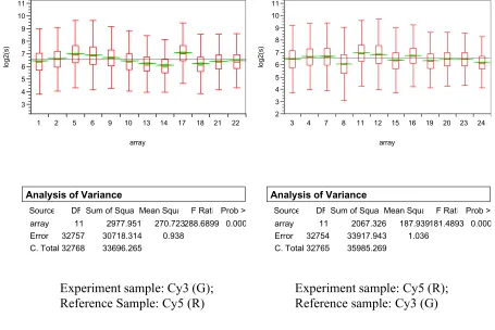
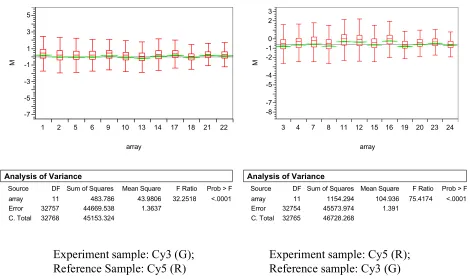
Assessing systematic errors

Data from kidney tissues across 24 arrays are analyzed to assess the array effect. Figures 1 and 2 show that there exists significant between array variation, both in terms of log2 based abso-lute signal intensity and in terms of log2 based ratio between R and G. In either case, the array

y_j ·

y

··

(57)

effect is highly significant as shown from the ANOVA tests. Similar analysis of data from liver and testis tissues also showed the significant variation between arrays.

To examine the block effect or between block variation within an array, data from array 1 in kidney tissue was plotted as shown in Figures 3 and 4. We can see there exists significant between block or between block variation within an array both in terms of log2 based absolute signal intensity (Figure 3) and in terms of log2 based ratio between R and G (Figure 4). Such effect is consistently significant in other arrays too.

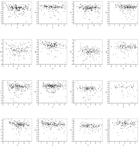
Figure 5 shows that log2 based R/G ratio varies as the average signal intensity of R and G changes. Instead of plotting R against G, transformed coordinates M and A are used, where M = log₂R/G and A = 1/2(log₂R + log₂G). An M vs. A plot is another representation of (R,G) data in

terms of the log₂ based R/G which is often the quantity of interest. It has the advantage of

detect-ing intensity dependent patterns in log ratios better than (log₂R vs. log₂G) coordinates (Dudoit et

al., 2000). We can see that in all of the blocks, the value of M varies as the value of A changes. Ideally, we would observe a horizontal line at M=0, which means at any value of average fluores-cent signal intensity of the two dyes, the ratio between the two dyes is consistently equal to 1. Fig-ure 5 also shows that such variation in M differs from one block to another which implies the normalization to remove such systematic dye incorporation variation needs to be done on a block by block basis.

(58)

dif-out. To see how effective a normalization step is, we also compared methods 1~5 with methods 6 and 7, where gene-based ANOVA tests are directly used, without the normalization step. Method 6 used log2 based ratios between the two dyes. The ratio is calculated as the fluorescent signal intensity of the experiment sample divided by fluorescent signal intensity from the reference sam-ple. Method 7 used absolute signal intensity values for the response variable to identify differen-tially expressed genes.

Normalization methods

Normalization method #1: Adjust for within block log ratio dependency on average intensity value using a local smoothing method, then adjust between array dispersion by standardization.

This method is very similar to the one implemented by Pritchard et al. (2001). To adjust the discrepancy in terms of dye incorporation between Cy3 (R) and Cy5 (G), a robust scatter-plot smoother lowess function is adapted to perform the local intensity dependent normalization (Dudoit et al., 2000; Yang et al., 2000). Instead of using R and G, transformed coordinates M and A were used, where M = log₂R/G and A = 1/2(log₂R + log₂G) (Dudoit et al., 2000).

We implement this approach with SAS procedure PROC LOESS (SAS Institute Inc., 1999b). In the LOESS procedure, a nonparametric method for estimating local regression surfaces is

implemented. For example, let be a regression function for on such that ,

where is the random error term. The idea is that near , a local approximation can be

obtained by fitting the regression lines to the data points within a chosen neighborhood of . The

chosen neighborhood represents a specified percentage of the all the data points around . This

g y_i x_i y_i = g x( ) ε_i + _i

ε_i x = x₀

x₀

(59)

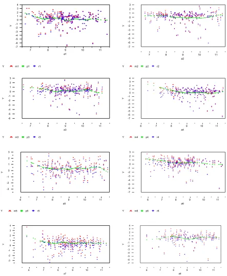
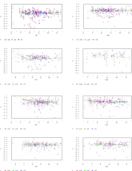
can be controlled by smooth option in PROC LOESS (Cohen RA, 1998). It controls the smooth-ness of the estimated line. While implementing a normalization step with the local smoothing technique, we also want to see how different settings of this option affect the normalization results and ultimately influence the number of genes and the actual genes identified to be differentially expressed between mice. Figure 6 shows the results from running this procedure within each

block in array 1, where points in red are observed values, points in green are predicted values,

‘s, from local smoothing fitting, and blue points are the residuals, ‘s.

When adjusting for log ratio dependency on average signal intensity within blocks, block means and array means are automatically adjusted to be at the same level, near zero. The next step is to adjust for data dispersion between arrays such that they are all on the same scale before applying gene-based ANOVA models. We have chosen to use array specific standard deviation to perform such adjustment, similar to the one used by Pritchard et al. in the paper where median of the deviation of the median was used.

Normalization method #2: Global normalization on log2 based ratios to adjust between block variation.

The block-specific mean is first subtracted from each ratio value and then standardized by

block-specific standard deviation. If let be the observed log ratio in block j of array i for gene

k, and let , represent the mean and standard deviation of block j of array i in terms of log

ratios, then normalized value for is:

y_i

yˆ_i eˆ_i

y_ijk

y_ij · sij

(60)

This procedure is done for each of the 16 blocks on each of the 24 arrays for a certain tissue. After the normalization procedure, all log ratios are adjusted to be with mean zero and standard devia-tion 1. Since this step is performed at the block level, between array variadevia-tion is thus automati-cally adjusted. Dependency of log ratio between two dyes on average signal intensity is not specifically adjusted, but dye effect is fit into the gene-based ANOVA model (See Equation 6).

Normalization method #3: Global normalization on logarithm of absolute value to adjust between block variation.

This method is very similar to method #2. The only difference is that ‘s here are the

log-arithms of absolute signal intensity values instead of log ratios. The same gene-based ANOVA models as in method #2 was subsequently applied, and again, the logarithm of absolute signal intensity value instead of the ratio was used.

Normalization method #4: Use ANOVA to normalize logarithms of absolute signal values, then fit residuals from normalization ANOVA with a gene-based ANOVA to identify differentially expressed genes (Wolfinger et al., 2001).

Based on the particular design in this experiment, we have adopted the following ANOVA model for data normalization. Effects that contribute to the systematic variation include array, block and dye. As proposed by Wolfinger et al., we have fit the data into a mixed model as shown below,

, (5)

y_abg