Solving Delay Differential Equations with
Constant Lags using RKCeM Method
Emimal Kanaga Pushpam A1, Vinci Shaalini J 2
Associate Professor, Department of Mathematics, Bishop Heber College, Tiruchirappalli, Tamil Nadu, India1 Department of Mathematics, Bishop Heber College, Tiruchirappalli, Tamil Nadu, India2
ABSTRACT: This paper presents RK method based on Centroidal mean for solving Delay differential equations with constant delays. The delay term is approximated by using linear and Lagrange interpolation.The effectiveness of this method has been illustrated with examples. The numerical results are also compared with RK method based on Arithmetic mean.
KEYWORDS: Delay differential equations, constant delay,multiple delays, IVP, RKAM, RKCeM. I. INTRODUCTION
Delay differential equations (DDEs) arise in population dynamics [1], control systems [2], chemical kinetics [3] and in many areas of Science and engineering. Recently there has been great interest in finding the numerical solutions of DDEs. Many numerical methods have been suggested for solving DDEs of first order as in [4-6]. Paul and Baker [7] discussed about the determination of stability regionof RK method for DDEs. Hu et al. [8] considered the stability of RK methods for DDEs with multiple delays.
Evans and Yaakub [9] have proposed the fourth order RK method based on Centroidal mean (RKCeM) for solving IVPs. Murugesan et al. [10] have applied RKCeM to solve second order IVPs.
In this paper the fourth order RKCeM method has been discussed for obtaining the numerical solution of first order DDEs. Here we consider the first order DDEs in the following form:
))
(
),
(
,
(
)
(
'
t
f
t
y
t
y
t
y
,t
t
0)
(
)
(
t
t
y
,t
t
0 if it has one delay only, or) ( ),..., (
), ( ), ( , ( ) (
' t f t y t y t 1 y t 2 y t n
y
,t
t
0)
(
)
(
t
t
y
,t
t
0if it has more than one delay term where
(
t
)
is the initial function. Here the delay terms
,
1,
2,...,
n are positive constants.Three numerical examples have been considered to demonstrate the adaptability of RKCeM to DDEs.stability for RKCeM have been discussed. In Section V, the numerical examples have been provided to illustrate the effectiveness of RKCeM.
II. RKCEM METHOD FOR ORDINARY DIFFERENTIAL EQUATIONS Consider the first order equation of the form
)
,
(
'
f
x
y
y
withy
(
x
0)
y
0.
The fourth order RKAM formula of the (n+1)th increment in y is computed as
2
2
2
3
4 3 3 2 2 1 1k
k
k
k
k
k
h
y
y
n n
3 1 3 1 13
2
3
i n i i i nAM
h
y
k
k
h
y
where
3
4 2 3 1 2 1
,
2
1
,
2
1
2
1
,
2
1
,
hk
y
h
x
f
k
hk
y
h
x
f
k
hk
y
h
x
f
k
y
x
f
k
n n n n n n n n
Evans and Yaakub have developed a new RK method of order four based on Centroidal mean in solving first order differential equations. The Centroidal mean of two points
y
1 andy
2is defined as2 2
1 1 2 2
1 2
CeM
y
y y
y
.
y
y
By replacing the AMin eqn. (2.1) by CeM, the fourth order RKCeM formula is written as
4 3 2 4 4 3 2 3 3 2 2 3 3 2 2 2 2 1 2 2 2 1 2 1 19
2
k
k
k
k
k
k
k
k
k
k
k
k
k
k
k
k
k
k
h
y
y
n n2 2 3 1 1 1 1 1
2
. .
3 3
i i i i
n n
i i i
k
k k
k
h
i e y
y
where 1
2 1
3 1 2
4 1 2 3
(
,
)
1
1
,
2
2
1
1
11
,
2
24
24
11
25
73
,
132
132
66
n n
n n
n n
n n
k
f x y
k
f x
h y
hk
k
f x
h y
hk
hk
k
f x
h y
hk
hk
hk
The Butcher array for RKCeM is
0
1
2
1
2
1
2
1
24
11
24
1
11
132
25
132
73
66
1
3
1
3
1
3
III. RKCeM METHOD FOR DELAY DIFFERENTIAL EQUATIONS Consider the first order DDE of the form
))
(
),
(
,
(
)
(
'
t
f
t
y
t
y
t
y
,t
t
0)
(
)
(
t
t
y
,t
t
0where
(
t
)
is the initial function and
is the delay term. When we adapt the fourth order RKCeM formulato DDE, we have
4 3
2 4 4 3 2 3 3
2
2 3 3 2 2 2 2
1
2 2 2 1 2 1 1
9
2
k
k
k
k
k
k
k
k
k
k
k
k
k
k
where
4
1
,
, (
) , (i 1,..., 4).
i n i n ij j n i
j
k
f x
c h y
h
a k y x
c h
The above RKCeM formula can also be extended to solve DDEs with multiple delays.
IV. CONVERGENCE AND STABILITY OF RKCeM
Order of Convergence of RKCeM:
When we use RKCeM formula to solve DDEs, the delay term
y
(
x
n
c
ih
)
need to be interpolated to approximate the value. Many techniques are available for the approximation.In this paper linear and Lagrange interpolation are used to approximate the delay term. The interpolation order have to be adapted to the order of the method.For any given RK method, its adaptation to DDEs by means of interpolation procedure has an order of convergence equal to
min
p q
,
where p denotes the order of consistency of the RK method and q is the number of support points of the interpolation procedure. (See [11])For linear interpolation we are using two support points so that the order of convergence of RK method is two (See [12]) which is less than the order of the RK method. For Lagrange interpolation we are using five support points so that the order of convergence of RK method is four for DDEs also.
Linear stability for RKCeM:
There are many concepts of stability of numerical methods to DDE, which depends on the test equation as well as the delay term involved.Here our attention is to a linear test equation with a constant delay
,)
(
)
(
)
(
'
x
y
x
y
x
y
,t
t
0)
(
)
(
t
t
y
,
t
t
0 where
,
R
,
0
and
is continuous.The Butcher array representation of RK method is of the form C A
bT
The stability function of s-stage RK method for ODE is given by
1(z)
1 zb
T,
r
I
zA
e
In the case of DDEs, we consider
Nh
whereN
is a positiveinteger.In this case whenu nh c h
i
is required a previous internal stage-valueY
n N i , is used. Here we consider the stability properties of a recurrence of the form1 1
1
1
(
)
(
)
T T
n n n N
y
hb
I
hA
e y
hb
I
hA
u
where
u
n N is a vector consisting of ‘back- values’u nh c h
i
. This can be expressed in a convenient form as1
1
(
)
(I
)
.
T
n n n N
y
r
h y
hb
hA
u
If we write
S
S
(
h
)
(
I
hA
)
1 and
n
Y
n,1,...,
Y
n,s
T,
the above can be written as Nn T n
n
r
h
y
hb
S
y
1
(
)
_We can express this as the recurrence:
1
n
X
nZ
n N
where
0
0
)
(
Se
h
r
X
and
hSA
S
hb
Z
T
0
0
.
This recurrence is stable if the zeros
iof the stability polynomial 1( , ; )
det
N N.
h
S
I
X
Z
The root condition for stability is the requirement that all the zeros
i ofS
h(
,
;
)
satisfy
i
1
, and if
i
1
then
iis semi-simple.The stability polynomial of RKAM is obtained as
2 3 4 2 3
5 5 1 4 1
2 2 3 4
3 1 2 1 1
( , ; ) 1 1
2 6 24 2 6
1 1
2 2 6 24
N N N
N N N
h h h h h
S h h h h h
h h h h
h h
and the stability polynomial of RKCeM is obtained as
2 3 4 5
2
5 5 1 4 1
2 3
3 1 2 1
37 2 11
1 1
2 3 24 5184 3 48
1 11 11
.
(
,
; )
N N NN N
h h h h
h h h h
h h h
S
h
h
V.NUMERICAL EXAMPLES Example 1
Consider the first order DDE with single delay
'( )
(
1)
( )
t,
1
0
y t
y t
y t
e
t
with exact solution
)
(
t
y
=
( 2 )
2 2
( 3 )
( 1
)
on
0,1
on
1, 2
2
2
on
2, 3
2
2
t
t
t
e
e
t
e
t
e
e
t
t
e
e
e
This problem is solved by RKAM and RKCeM by using linear interpolation and Lagrange interpolation for the delay term with
1.
The absolute error results are shown in the following Tables 1 and 2.Table 1 Results of Example 1 (Linear Interpolation) Time Absolute Error
(RKAM)
Absolute Error (RKCeM) 0.50 1.99e-006 2.32e-006 1.00 5.27e-006 6.15e-006 1.50 7.71e-006 8.81e-006 2.00 1.27e-005 1.44e-005 2.50 1.79e-005 2.05e-005 3.00 2.61e-005 3.00e-005
Table 2 Results of Example 1 (Lagrange Interpolation)
Time Absolute Error (RKAM)
Example 2:
Consider the system of first order DDE with single delay
1
0
,
)
3
.
0
(
)
(
)
(
'
)
(
)
(
'
)
(
)
(
'
) 3 . 0 ( 1
1 3
3 2
2 1
t
e
t
y
t
y
t
y
t
y
t
y
t
y
t
y
t
with initial functions
0
,
)
(
;
)
(
;
)
(
2 31
t
e
t
y
e
t
y
e
t
y
t t twith exact solutions
t t
t
e
t
y
e
t
y
e
t
y
1(
)
;
2(
)
;
3(
)
This problem is solved by RKAM and RKCeM by using linear interpolation and Lagrange interpolation for the delay term. The absolute error results are shown in the following Tables 3 and 4.
Table 3 Results of Example 2 (Linear Interpolation)
Time
Absolute Error (RKAM) Absolute Error (RKCeM)
y1 y2 y3 y1 y2 y3
0.20 3.57e-009 5.27e-008 5.10e-007 3.56e-009 5.26e-008 5.10e-007 0.40 2.72e-008 1.98e-007 9.24e-007 2.72e-008 1.97e-007 9.24e-007 0.60 8.75e-008 4.17e-007 1.25e-006 8.75e-008 4.17e-007 1.25e-006 0.80 1.98e-007 6.94e-007 1.50e-006 1.98e-007 6.93e-007 1.50e-006 1.00 3.68e-007 1.01e-006 1.66e-006 3.68e-007 1.01e-006 1.66e-006
Table 4 Results of Example 2 (Lagrange Interpolation)
Time
Absolute Error (RKAM) Absolute Error (RKCeM)
y1 y2 y3 y1 y2 y3
0.20 8.57e-013 8.58e-013 8.43e-013 3.44e-015 3.44e-015 3.44e-015 0.40 1.40e-012 1.41e-012 1.35e-012 6.99e-015 6.99e-015 6.99e-015 0.60 1.72e-012 1.75e-012 1.50e-012 1.90e-014 1.89e-014 1.93e-014 0.80 1.86e-012 1.98e-012 1.37e-012 2.58e-014 2.57e-014 2.50e-014 1.00 1.87e-012 2.16e-012 1.07e-12 2.87e-014 2.90e-014 2.65e-014
Example 3:
Consider the system of first order DDE with multiple delay
1 5 3 2 1 2 3 3 1
4 5 4 5 1
1
1
' ( )
(
1)
(
1);
' ( )
(
1)
(
);
' ( )
(
1)
(
)
2
2
' ( )
(
1)
(
1);
' ( )
(
1)
0
y
t
y t
y t
y
t
y t
y t
y
t
y t
y t
y
t
y t
y t
y
t
y t
for t
with analytical solutions for0 1 2
t
1 1 1
( )
2 2 2
1 2 3
2
4 5
( )
cos
;
( )
2
2;
( )
cos
1
sin(1);
1
1
( )
;
( )
1
2
2
t
t t
t t
y t
e
t
e
y t
e
e
y t
e
t
e
y t
e
e
y t
e
e
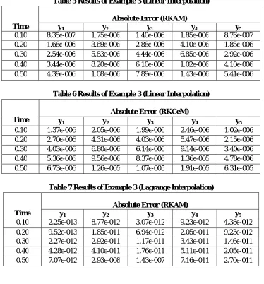
This problem is solved by RKAM and RKCeM by using linear interpolation and Lagrange interpolation for the delay term. The absolute error results are shown in the following Tables 5 - 8.
Table 5 Results of Example 3 (Linear Interpolation)
Time
Absolute Error (RKAM)
y1 y2 y3 y4 y5
0.10 8.35e-007 1.75e-006 1.40e-006 1.85e-006 8.76e-007 0.20 1.68e-006 3.69e-006 2.88e-006 4.10e-006 1.85e-006 0.30 2.54e-006 5.83e-006 4.44e-006 6.85e-006 2.92e-006 0.40 3.44e-006 8.20e-006 6.10e-006 1.02e-006 4.10e-006 0.50 4.39e-006 1.08e-006 7.89e-006 1.43e-006 5.41e-006
Table 6 Results of Example 3 (Linear Interpolation)
Time
Absolute Error (RKCeM)
y1 y2 y3 y4 y5
0.10 1.37e-006 2.05e-006 1.99e-006 2.46e-006 1.02e-006 0.20 2.70e-006 4.31e-006 4.03e-006 5.47e-006 2.15e-006 0.30 4.03e-006 6.80e-006 6.14e-006 9.14e-006 3.40e-006 0.40 5.36e-006 9.56e-006 8.37e-006 1.36e-005 4.78e-006 0.50 6.73e-006 1.26e-005 1.07e-005 1.91e-005 6.31e-005
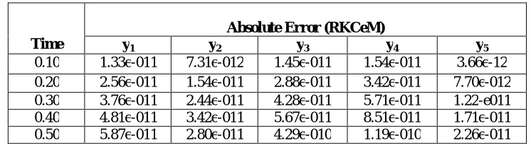
Table 7 Results of Example 3 (Lagrange Interpolation)
Time
Absolute Error (RKAM)
y1 y2 y3 y4 y5
Table 8 Results of Example 3 (Lagrange Interpolation)
Time
Absolute Error (RKCeM)
y1 y2 y3 y4 y5
0.10 1.33e-011 7.31e-012 1.45e-011 1.54e-011 3.66e-12 0.20 2.56e-011 1.54e-011 2.88e-011 3.42e-011 7.70e-012 0.30 3.76e-011 2.44e-011 4.28e-011 5.71e-011 1.22-e011 0.40 4.81e-011 3.42e-011 5.67e-011 8.51e-011 1.71e-011 0.50 5.87e-011 2.80e-011 4.29e-010 1.19e-010 2.26e-011
VI. CONCLUSION
In this paper, RKCeM formula has been adopted to solve the delay differential equations with constant lags. The effectiveness of this approach has been illustrated via examples of DDE with single delay and multiple delays. To interpolate the delay term, both linear interpolation and Lagrange interpolation have been considered here. The numerical outcomesalso have been compared with RK method based on arithmetic mean. From the numerical results, it is observed that the RKCeM method is well suitable for solving DDEs. It also suggests that the best results can be obtained when we use Lagrange interpolation with suitable number of support points for getting fourth order convergence.
REFERENCES
[1] Kuang, Y.,“Delay Differential Equations with Applications in Population Biology”, Academic Press, Boston, San Diego, New York, 1993.
[2] Fridman, E.,Fridman, L.,and Shustin, E.,“Steady Modes in Relay Control Systems with time delay and periodic disturbances”, Journal ofDynamical Systems Measurement and Control, Vol. 122, pp. 732-737, 2000.
[3]Epstein, I.Y., and Luo, “Differential delay equations in chemical kinetics: Non-linear models; the cross-shaped phase diagram and the Oregonator”, Journal of Chemical Physics, Vol. 95 pp. 244-254, 1991.
[4] Van der Houwen P.J., and B.P. Someijer, “Explicit Runge-Kutta (Nystrom) methods with reduced phase errors for computing oscillating solutions ”, SIAM Journal on Numerical Analysis, Vol.24, No.3, pp.595-617, 1987.
[5] Imoni, S.O., Otunta, F.O. ,and Ramamohan,T.R., “Embedded implicit Runge-Kutta Nystrom method for solving second order differential equations”, International Journal of Computer Mathematics, Vol. 83, No. 11, pp.777-784, 2006.
[6] Senu, N., Sulieman,M., and Ismail,F., “An embedded explicit Rungekutta-nystrom method for solving oscillatory problems", Physica Scripta, Vol. 80, No. 1, Article 1D015005, 2009.
[7] Christopher T.H. Baker and Christopher A.H. Paul, “Computing stability regions- Runge-Kutta methods for delay differential equations”, Mathematics Department, University of Manchester, UK, IMA Journal of Numerical Analysis, Vol. 14, pp. 347-362, 1994.
[8] Guang-Da Hu, Guang-Di and Meguid, S. A., “Stability of Runge-Kutta methods for delay differential systems with multiple delays”, IMAJournal of Numerical Analysis, Vol. 19, pp. 349 – 356, 1999.
[9]Evans, D.J. and Yaakub, A.R.,“A new 4th order Runge-Kutta Method based on the Centroidal Mean (CeM) formula”, Computer studies
851Department of Computer Studies, University of Technology, Loughborough, U.K., 1993.
[10] Murugesan, K., Paul Dhayabaran, D., Henry Amirtharaj, E.C., and David J.Evans, “Numerical Strategy for the system of second orderIVPs using RK method based on Centroidal Mean”, Inter. J. Computer Math., Vol. 80(2), pp. 233-241, 2003.
[11]In’t Hout, K. J. , “Convergence of Runge-Kutta method for Delay differential equations”, BIT Numerical Mathematics, Vol. 41, pp. 322-344, 2001.