Volume 2009, Article ID 804621,10pages doi:10.1155/2009/804621
Research Article
A Scheduling Algorithm for Minimizing the Packet Error
Probability in Clusterized TDMA Networks
Arash T. Toyserkani, Mats Rydstr¨om, Erik G. Str¨om, and Arne Svensson
Department of Signals and Systems, Chalmers University of Technology, 412-96 G¨oteborg, Sweden
Correspondence should be addressed to Arash T. Toyserkani,[email protected]
Received 1 December 2008; Revised 18 April 2009; Accepted 25 July 2009
Recommended by Wing-Kin Ma
We consider clustered wireless networks, where transceivers in a cluster use a time-slotted mechanism (TDMA) to access a wireless channel that is shared among several clusters. An approximate expression for the packet-loss probability is derived for networks with one or more mutually interfering clusters in Rayleigh fading environments, and the approximation is shown to be good for relevant scenarios. We then present a scheduling algorithm, based on Lagrangian duality, that exploits the derived packet-loss model in an attempt to minimize the average packet-loss probability in the network. Computer simulations of the proposed scheduling algorithm show that a significant increase in network throughput can be achieved compared to uncoordinated scheduling. Empirical trials also indicate that the proposed optimization algorithm almost always converges to an optimal schedule with a reasonable number of iterations. Thus, the proposed algorithm can also be used for bench-marking suboptimal scheduling algorithms.
Copyright © 2009 Arash T. Toyserkani et al. This is an open access article distributed under the Creative Commons Attribution License, which permits unrestricted use, distribution, and reproduction in any medium, provided the original work is properly cited.
1. Introduction
One of the problems with many wireless networks today is energy consumption, stemming from the fact that modern radio transceivers are often battery powered, and, hence, energy is a scarce resource that needs to be conserved as much as possible. Complexity is another important issue, since, many wireless network applications require the size and cost of individual network nodes to be kept at a minimum. One important example of the above is wireless sensor networks (WSNs) [1, Chapter 1], that have lately received considerable attention, both from industry and academia.
In order to conserve energy, the number of packet retransmissions in the network should be kept as low as possible. High packet-loss probability is undesirable, since it can potentially cause a high number of packet retransmissions. Another important factor in preserving energy is the duty cycle of individual nodes. For instance, recent work on energy consumption in WSNs has shown that most wireless sensor devices consume almost as much energy when listening to the wireless channel, or even being
in idle mode, as they do when actively transmitting a packet [1, Chapter 2]. From this perspective, a synchronized time slotted medium access (MAC) scheme (TDMA) where nodes can sleep for extended periods of time seems preferable both from interference and duty-cycle points of view. However, interference will still be present if two or more networks, or “clusters” of nodes, are colocated in close vicinity of each other.
One frequently occurring drawback with MAC design proposals is that overly simplistic propagation models are used, for example, not accounting for Rayleigh fading effects. For instance, channel assignment problem in wireless net-work is often addressed by modelling the netnet-work as directed graph [6], [7, Section III-A-1], and [8]. This assumption is not suitable in fading channels where the link gains vary over time, unless all the instantaneous link gains are frequently measured and made available to the scheduler, resulting in much added overhead and complexity.
In this work, we include Rayleigh fading and log-distance path loss in the system model and propose a TDMA-type MAC mechanism that jointly schedules transmissions between nodes and cluster heads with the objective to minimize the average packet error rate (PER), (The packet error rate is assumed to be equal to the block error rate. However, in general, they are not equal but closely related.) that is, to maximize the total network throughput. We make the assumption that all nodes have a fixed output transmission power and formulate the scheduling problem as an integer programming problem, more specifically an assignment problem.
Similar approaches are taken in [9, 10], where joint opportunistic power scheduling and rate control problems are considered. Our work differs from [9,10], and references cited therein, on three main points (a) Instead of allowing a smooth tuning of transmitter output powers, we impose an on-offconstraint on transmitters. One of the main reasons is that power consumption is sometimes only weakly correlated with transmit power [1, Chapter 2]. (b) Instead of the signal to interference and noise ratio (SINR), we consider the PER (a nonlinear function of SINR) to be the main optimization objective. While the PER is a more relevant measure, the SINR is often preferred in the literature due to the lack of a tractable analytical solution for the PER for a wide range of different modulations, coding methods, and fading channels [11]. To overcome this, a closed-form formula for estimation of the PER in block faded Rayleigh channels in presence of interference is derived and shown to be highly accurate. Finally, (c) in order to make the sleep time as long and uninterrupted as possible, we do not schedule nodes on a slot-by-slot basis. Instead, we schedule all slots in a frame in one run of the algorithm such that no node receives more than one slot.
The remainder of this paper is organized as follows. In Section 2, we define the network and interference model and state additional assumptions on the system. The utility function based on our analytical approximation of PER is introduced inSection 3. The interference model is later used in the proposed MAC algorithm, that is derived inSection 4. The proposed algorithm is analyzed and evaluated through computer simulation inSection 5, and we conclude the paper inSection 6.
2. System Model
LetMtransceiver nodes andKdata sinks be deployed over a bounded area. The nodes are indexed by integers 1, 2,. . .,M,
and are clustered into K sets {Ci}Ki=1. Let a frame be an
interval of time divided into W slots, indexed by w ∈ {1,. . .,W}, and letSw be the set of nodes, one from each cluster, scheduled for transmission in slot w. If there are fewer nodes in a cluster than the number of slots in a frame, “dummy” nodes at infinite distance from all sinks are added to the cluster. It is worth noting that a very largeWmay result in a trivial interference-free schedule where in each time slot only one real node is scheduled with dummy nodes from all other clusters. However, settingWarbitrarily large is not possible in a majority of practical systems as it also results in a large network delay and a low network throughput. The problem of how to adjustW and how to select a subset of nodes when the number of nodes per cluster is larger than Wis not considered here.
Based on these assumptions, each cluster contains exactly W nodes. In each frame, allW nodes in each cluster are to be scheduled such that no more than one node from each cluster is scheduled in a given slotw, and a node can only be scheduled once per frame. A schedule{S1,S2,. . .,SW}that satisfies these conditions is called a feasible schedule. Each cluster is assumed to have a dedicated sink node, or cluster head. Similar to a Bluetooth system [1, Chapter 5], the cluster head is the receiver of all transmissions from all nodes in a cluster. The scheduling is performed by a central entity that is connected to all sinks. While these settings resemble a cellular network architecture, the scheduling techniques developed for cellular networks are not applicable here. This is due to the fact that in cellular networks, power and rate control are essential part of the scheduling problem. While in wireless sensor networks, the on-off power control is preferred, which results in a fundamentally different problem formulation.
We assume the packet length is fixed, and that all cluster heads are coarsely synchronized on a packet level, so that transmissions in a given slot takes place at approximately the same time in all clusters. However, synchronization errors among clusters are considered in the numerical evaluations of the proposed algorithm (Section 5).
2.1. Interference Model. The instantaneous received power from the nodeiat sinkkis represented byPi,kand is defined as
Pi,k=κi,kPi,k, (1)
With these assumptions, the instantaneous SINR for the
where PNk denotes the (known) thermal noise power at
cluster headk.
3. Utility Function
It is shown in [11] that in an interference free environment, the PER of block coded packets in block faded Rayleigh channels can be accurately approximated by a simple SNR threshold. That is each received packet is considered to be successful if the instantaneous SNR is above a given threshold
Θ, and lost otherwise. Hence, the PER in the block faded Rayleigh channels is approximated by [11]
Ploss
wherePloss(Γ) is the PER estimate based on SNR threshold
model and Γis the average SNR. Similar results for turbo coded packets are reported in [13].
In this section, we examine if applying a similar method in presence of interference results in an accurate approxima-tion of PER. In TDMA systems with block fading channels, SINR is constant during one time slot (if the intercluster synchronization error is small). Therefore, applying the threshold method results in
Since all fading coefficients are i.i.d. unit-mean exponential random variables, we have, as shown in the appendix,
Ploss(k,Sw)=1−
The accuracy of this model is verified by comparing the PER for the node-sink link of nodem, denoted byPe,m, withPloss
for the same link. An analytical expression forPe,m can be obtained by integrating the instantaneous PER over the SINR variations where the instantaneous PER for nodem=Sw(k) is given by correction capability (in number of bit errors). Interested readers are referred to [14] and references cited therein, for more information regarding the block error probability of various coding and decoding methods.
Since the closed-form analytical solution to Pe,m is untractable [11], Monte-Carlo simulation is used in this paper to estimatePe,m. The required statistics were obtained through simulations of 200 randomly generated networks. For each the node-sink link,Pe,m is obtained by averaging over 1000 Rayleigh fading realizations. The other simulation parameters can be found inSection 5.
InFigure 1, we plot the cumulative distribution function (CDF) of the differenceη=Pe,m−Plossevaluated for all links
in all networks. We see that, for a correctly chosen threshold, in this caseΘ=4.82 dB, the error is quite small. We also note that variations as large as±2 dB in the threshold increases the error, but not significantly, and hence the packet-loss model is not overly sensitive to the choice of threshold.
Finally, we note that the choice ofΘonly depends on the modulation format, that is, BPSK, the receiver architecture, the packet length, and the properties of the code. The threshold does not depend on the network configuration and layout, that is,K,M, and so forth. Hence the threshold can be decided prior to network deployment, and does not need to be reconfigured if the network configuration changes. For methods of findingΘ, interested readers are referred to [11]. To isolate the effect of the proposed Ploss formula, the
reliability, or “utility”, of a link from nodeSw(k) to cluster headk, is defined asUk(Sw)=1−Ploss(k,Sw). Adding more terms toUk(Sw) does not change the optimization algorithm inSection 4as long as utility of each schedule can be obtained independently of other schedules.
out from the summation in (7). The inclusion of dummy nodes in the analysis has some interesting implications. A cluster will have dummy nodes if it has more time slots than nodes. The schedule for the dummy nodes then indicates the best time slots for radio silence in the cluster from a global network perspective.
The utility functionU(Sw) in (7) does not necessarily need to consider all clusters. The throughput and its subsequent optimization from a subset of clusters’ point of view are obtained by simply removing appropriate terms from the sum in (7). The implications of this are analyzed inSection 5. We also emphasize that maximizing the utility function in (7) is different from maximizing the average SINR. With the utility in (7), increasing the SINR for a node beyond the point where Ploss ≈ 0 does not increase the
utility significantly. Conversely, the cluster utility does not change much if the SINR for a node withPloss≈1 is further
decreased.
4. Medium Access Control
The aim of the proposed Medium Access Control (MAC) layer is to schedule node transmissions such that the average probability of a successful packet delivery in the network is maximized. Due to the assumed slotted MAC scheme, this will also maximize the network throughput. We defineAas a set of all feasible slot schedules, that is,A= {{c1,. . .,cK}:
c1 ∈ C1,. . .,cK ∈ CK}. We also define Am as a set of feasible schedules where nodemhas been scheduled, that is,
Am= {a∈A:m∈a}.
The MAC problem for theKclusters{Ci}Ki=1andWtime
slots is then
max
{S1,...,SW}
W
w=1
a∈A
U(a)ISw,a
such that
(A) a∈A
ISw,a=1, ∀w∈ {1,. . .,W},
(B) W
w=1
a∈Am
ISw,a=1, ∀m∈ {1,. . .,M}.
(8)
Here, and throughout the rest of this work,Ia,bis an indicator function that is unity whena=band zero otherwise. TheW constraints in (A) ensures thatSw∈A, for allw=1,. . .,W. That is,Sw is a feasible slot schedule. TheM constraints in (B) ensure that all nodes are scheduled in exactly one slot. Hence, (A) and (B) are satisfied if and only if{S1,. . .,SW}is a feasible schedule.
As the number of nodes and clusters in the network grows, the complexity of a brute-force solution to (8) quickly becomes prohibitive. In fact, there are as many as (W!)K different feasible schedules to choose from.
4.1. MAC Problem for Two Clusters. Since we assume no time dependence, the utility functionU(Sw) only depends on the coscheduled nodes in the slot schedule Sw and not on the specific slot w. Hence, a permutation of slot schedules in a global schedule {S1,. . .,SW}will not affect the utilityWw=1U(Sw). We can therefore arbitrarily choose any feasible schedule for nodes in, for example, clusterC1,
without loss in maximum achievable utility. After fixing the schedule{Sw(1)}Ww=1 for nodes in C1 in a two-cluster
network, the MAC problem in (8) reduces to the two-dimensional assignment problem:
max
{S1(2),...,SW(2)}
W
w=1
c2∈C2
U({Sw(1),c2})ISw(2),c2
such that
(A) c2∈C2
ISw(2),c2=1, ∀w∈ {1,. . .,W},
(B2)
W
w=1
ISw(2),c2=1, ∀c2∈C2.
(9)
Unlike the case of a multidimensional assignment problem, efficient algorithms exist that solve (9) in polynomial time such as maximum weight matching problem on bipartite graph [15]. We use the auction algorithm, due to Bertsekas [16], [17, Chapter 6], briefly described below.
Consider problem (9), where the schedule for nodes in
C1, that is, {Sw(1)}Ww=1, is fixed and known. The auction
algorithm for solving this problem is as follows. (a) Envision the nodes inC2as objects on sale at an auction, and envision
the slots as buyers at the auction. Initially, the asking prices
{pc2}c2∈C2 of the objects on sale are set to zero. (b) Let each slot w successively “place a bid” on the node i =
arg maxc2∈C2{U({Sw(1),c2})− pc2}, that is, the node that yields the highest net value vi = U({Sw(1),i})− pi for slot w. (c) When a node is bid upon, its asking price pi is raised byvi−zi+β, whereβ > 0 is a small number, and
zi=maxc2∈C2,c2=/i{U({Sw(1),c2})−pc2}, that is, the second best net value for slotw. The reason for the additional small increase in price,β, is to prevent ties among buyers, a topic further discussed in [17]. In this paper we letβ=1/W. (d) The auction continues until all nodes have received at least one bid, at which point a solution to (9) has been found.
Although of little consequence for the development here, it is interesting to note that the auction algorithm is actually a dual method on its own. It can be shown that when the auction algorithm terminates, the node asking prices solves
min
{pc2}c2∈C2 W
w=1
sup c2∈C2
U({Sw(1),c2})−pc2
+
c2∈C2
pc2, (10)
to within any >0 of the optimal value (depends on the choice ofβ). This is, in fact, the dual problem to (9), after relaxation of constraints on nodes inC2.
4.2. MAC Problem for Arbitrary Number of Clusters. It was noted above that the complexity of a brute-force solution to (8) grows quickly withW andK. However, if a relaxed problem, that is, the maximization of a Lagrangian, can be easily solved, and we also have access to a good method that converts a solution to the relaxed problem into one that is primal feasible, then experience with similar types of combinatorial optimization problems; see, for example, [9, 10, 17–19], and references cited therein, gives that an iterative solution of the dual problem often yields a near optimal, or even an optimal solution to the primal problem. Hence, the algorithm we propose is an iterative algorithm similar to one in [18], where each iteration involves the following three steps. (1) Given a vector of dual variables, a relaxed version of (8) is solved. (2) A primal feasible schedule is constructed from the solution to the relaxed problem and the vector of dual variables. (3) If the obtained primal solution is found to be unsatisfactory, then the dual variables are updated, and we iterate again.
4.2.1. The Relaxation Step. We relax constraints on nodes in C3,C4,. . .,CK in (8). Let μcp denote the dual variable
associated with nodecp∈Cp. The dual function is then
qµ= feasible schedule for the nodes in, for example,C1, without
loss in maximum achievable utility. Let V(2)(w,c
2) =
supc3∈C3,...,cK∈CK{U({Sw(1),c2,. . .,cK})−μc3· · ·−μcK}, then
the problem in (11) is equivalent to
qµ=
Hence, for a given vector of dual variablesµ, this problem is a two-dimensional assignment problem which is easily solved, as was shown inSection 4.1. We note that, to compute V(2)(w,c
2), a search overWK−2slot assignments is necessary.
In the scenarios considered in this work, an exhaustive search is feasible. However, larger networks may require the addition of more advanced search methods, such as branch and bound techniques, further discussed inSection 5.
4.2.2. A Method for Generating Feasible Schedules. When solving (12), we implicitly obtain a feasible scheduling of nodes from clusters C1 and C2. A feasible schedule that
also includes nodes from remaining clusters must now be generated. In general, a schedule that is feasible for nodes in
C1,C2,. . .,Cr−1, forr=3, 4,. . .,K, can be extended into one
that is feasible also forCrby fixing the schedule for nodes in
C1,C2,. . .,Cr−1and then running an auction algorithm for
the nodes inCrwith modified utilities
V(r)(w,cr)= sup
After enforcing primal constraints on nodes in all clusters up to and includingCK, a feasible schedule has been generated from the solution to (11), and we can compute its primal objective function value using (8).
4.2.3. Algorithm Termination Criteria. By the weak duality theorem [19, Chapter 6], we have that, for any feasible schedule{S1,S2,. . .,SW}, and anyµ,
We denote the optimal primal objective function value by f, and the objective function value computed at iteration νby f(ν). Then, at iterationi,
the duality gap of iteration i, and it upper bounds the distance from the so far best found primal objective function value to the supremum of the primal objective function. A measure of the quality of the best found solution up to iterationiis the relative duality gap, given by
Δ(i)=minν∈{0,...,i}q
4.2.4. Dual Variable Update Step. If a satisfactory schedule has not yet been obtained, we update dual variables inµ. We use the heuristic “price-update” method proposed in [18], which is loosely based on the subgradient method [19] and has been shown to perform well for similar problems. We only give a brief overview of the update method here, and refer to [18] for the details.
After step (1) in iteration i, a node ck ∈ Ck will be temporarily “scheduled” ingck slots. Clearly, the scheduling
constraint is only satisfied if and only if gck = 1. In step
(2), the constraints will be enforced, cluster by cluster, by successive auctions. Letpckbe the price of the nodeckafter
the auction. We form three vectors,µ(ki) ∈ RW,g(i) k ∈ ZW, andp(ki)∈RW, whose elements areμ(i)
ck (the dual variable for
nodeckat iterationi),gc(ki), andp (i)
ck, respectively. The update
rule for the dual variables at iterationiis then
µ(i+1) p, · denotes Euclidean norm, denotes element-wise multiplication, and auction algorithm to enforce constraints on nodes inCk.
Intuitively, this dual variable update approach can be interpreted as follows. If, after fixing the schedule for clusters
C1 to Ck−1, two or more slots have a given node in Ck as their preferred choice in terms of interference conditions, then the “price” of this node is increased in future iterations of the algorithm. If there exist a node that no slot has as its preferred choice, then the price of this node is reduced. This way, solutions to the relaxed problem (11) that violates constraints in (8) are penalized.
For further examples of this dual method, although in a different application, we refer to [18] and references cited therein. A flowchart of the proposed algorithm is shown in Figure 2.
Fix schedule also forC3 using the auction
Figure2: Flowchart of the proposed algorithm.
5. Numerical Analysis and Discussion
5.1. System Setup. We consider a short-range clustered WSN, where all transceiver nodes use BPSK signalling with a fixed output powerP. To simplify our simulations, shadow fading is ignored and the average received powerPi,kis modelled by the log-distance path-loss model as follow:
Pi,k=P0
P0 is the average received power at distance d0. In the
simulations,P0/PN = 10 dB at reference distanced0 =1 m
and the path-loss exponent isα = 4. All links are affected by Rayleigh fading with unit power gain, that is assumed to be independent between links. We assume that thermal receiver noise and interference are both Gaussian with zero mean. A simple t = 5 bit error correcting block code with block length L = 800 bits is used by all nodes. One codeword is transmitted in each time slot, it occupies the entire slot, and the cluster head uses hard-decision decoding of codewords. All nodes are assigned one slot per frame, and this slot assignment does not change between frames in the simulation. We assume that the frame of clusteri starts at global timeT+ωi, where the synchronization errors{ωi}Ki=1
are i.i.d. zero-mean Gaussian with standard deviationσω. An example network schedule withW =3 slots and|Ck| =3 nodes per cluster (k=1, 2, 3) is shown inFigure 3, wheresk,w denotes the node inCkscheduled in slotw,Lis the number of symbols per packet, and Ts is the symbol duration. We remark that robustness to cluster synchronization errors can of course be increased if guard intervals are introduced between slots in the frame structure.
Frame duration=WLTs ω1
ω2
ω3
S3(1) S1(1) S2(1) S3(1) S1(1) S3(2) S1(2) S2(2) S3(2) S1(2)
S3(3) S1(3) S2(3) S3(3) S1(3) T
Figure3: Example of cluster frames and synchronization errors.
we first manually deploy K cluster heads at coordinates
{(xi,yi)}Ki=1. The node coordinates in thekth cluster is drawn
as |Ck| realizations from a circular Gaussian distribution with mean equal to the coordinates of thekth cluster head and standard deviation σR. The distance between cluster heads, σR,α, and P0/PN together determines the expected SINR conditions in the network. For a fixed αandP0/PN, a network with sparsely deployed cluster heads and small σR on the average experiences less intercluster interference than a network with more dense cluster heads and/or higher σR.
For notational convenience, we define a constant trans-mission range R, which is the range where the packet error rate (PER) goes above 10−2 in absence of fading and interference. In all simulated scenarios discussed below, cluster heads were deployed on the corners of a square with sideR, that is, at (0, 0), (R, 0), (0,R), and (R,R). Each of the K =4 clusters has 5 nodes, and there areW = 6 slots in a frame, which implies that each cluster has one dummy node. The proposed scheduling algorithm was run until the relative duality gapΔ(i)≤10−3, see (16), or until a maximum of 300 iterations.
5.2. Convergence Properties of the Proposed Algorithm and Some Remarks on Complexity. The convergence of Lagrangian relaxation method that is used in this work is only guaranteed if a strong duality property can be proven. Since strong duality of the general method used here is still an open problem in the literature, the convergence of this application of the optimization method is not proven either. Nevertheless, the dual function, defined in (11), provides an upper bound to the primal which implies that even if the algorithm fails to converge in some scenarios, the maximum potential gain of an unknown optimal solution over the best known schedule is always obtained. This result has significant practical importance as it can be used to trade performance for complexity, especially when working with iterative scheduling approaches.
In this section, the convergence properties of the pro-posed algorithm are studied by extensive simulations. During the simulations, the best achieved utilities U(1), U(5), and
U(300) after at most 1, 5, and 300 iterations, respectively,
were stored. An upper bound on achievable utility in each network was also computed. This bound was computed as (1 +Δ(300))U(300), where Δ is the relative duality gap
defined in (16). To investigate the convergence properties of the proposed algorithm, we computed the relative utility difference (i) = (1/M)((1 +Δ(300))U(300) − U(i))/U(i),
for i = 1, 5, 300. This difference indicates how close to the optimal solution the algorithm is after i iterations. If
= 0, then the optimal schedule has been found, while, if > 0, an average relative increase of in utility per node could possibly be achieved by additional iterations of the algorithm. We define (0) to be the relative difference between a random scheduling (with utility U(0)) and the
upper bound.
The CDFs of (i),i = 0, 1, 5, 300, for cluster densities σR = R/2 and σR = R/4, are plotted inFigure 4. We note that the achieved objective function value is very close to its upper bound after at most the maximum 300 iterations. In fact, in our simulations, the (300) was almost always less than 0.001. Hence, the algorithm performs well in terms of convergence. Additionally, Figure 4 indicates that convergence is quite fast, that is, the distance to the upper bound is reasonably small already after only a few iterations. The results obtained after a single iteration deserves some special attention. It appears that a reduced complexity “greedy” algorithm that only iterates once, that is, executes K−1 consecutive auction algorithms, can be used without a significant degradation in performance. This conclusion is of great importance in networks where complexity is a limiting factor. The overall complexity of the proposed algorithm mainly depends on W, K, and the number of iterations the algorithm spends before termination. As noted in Section 4.2, there are (W!)K different feasible schedules to consider. However, the proposed algorithm only investigates a small subset of all possible feasible schedules.
Empirical tests on a personal computer have indicated that networks of up toK = 10 clusters, each withW = 7 nodes (e.g., the maximum number of slaves in a Bluetooth network), are manageable with the proposed algorithm. The part of the algorithm that introduces most complexity is the search for V(2)(w,c
2) in (11), which is implemented here
as an exhaustive search over theWK−2possible relaxed slot
w assignments. If larger networks than K = 10,W = 7 is required, then more advanced search methods must be considered.
Since all the nodes in every clusters are scheduled after a single run of the algorithm, the update frequency of the schedules depends only on the mobility, that is, the rate that average powers vary. In the low mobility sensor networks considered in this paper, the frequency of schedule update is substantially lower than the schedule usage time and therefore, the communication overhead cost of the proposed algorithm in these scenarios is negligible.
0.2 0.4 0.6 0.8 1
Pr
{
<
abscissa
}
0 0.0005 0.001 0.0015 0.002 0.0025 0 0.01 0.02 0.03
(0),σR=R/2 (0),σR=R/4 (1),σR=R/2 (1),σR=R/4
(5),σR=R/2 (5),σR=R/4 (300),σR=R/2 (300),σR=R/4
Figure4: Algorithm convergence,(i)=(1/M)(((1 +Δ(300))U(300)−U(i))/U(i)).
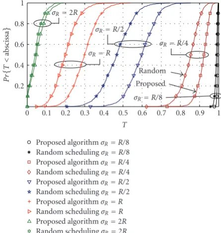
threshold was again set toΘ=4.82 dB. Two schedules were generated for each network layout, one using the proposed algorithm, and one random but feasible schedule. For each network and schedule, in addition toPe,m for all nodes, we also compute the normalized network throughputT, given byT=M−1Mm=1(1−Pe,m).
The CDF of network throughput is plotted inFigure 5 for the two scheduling approaches and for three different cluster densities. As expected, the increase in throughput is the highest when interference is significant, but SINR is still sufficient for communication. The increase in throughput is slim for scenarios where the overall SINR conditions in the network are either very good, or very bad, compare with the results forσR=R/8 andσR=2R.
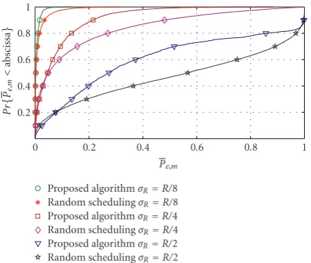
To investigate the impact of the proposed scheduling approach on individual nodes, we also plot the CDF of Pe,m evaluated for all nodes in all networks (Figure 6). It is interesting to note that the proposed algorithm reduces the number of nodes with relatively highPe,m, at the expense of nodes that have aPe,mcloser to zero. Although this effect is not significant, it is noticeable for the case ofσR=R/2.
As mentioned inSection 3, the utility measure in (7) does not need to encompass all clusters. For instance, suppose we control a number of node clusters that are deployed in the vicinity of a number of “alien” clusters with a fixed TDMA schedule that we have knowledge of, but cannot control. We would like to maximize the packet delivery ratio in our network, but we may not want to do so at the expense of the “alien” clusters, that could for instance be a legacy system. The impact on PER in clusters that are not accounted for by the utility function was evaluated in 200 networks. The parameters used in Figures 5 and6, with σR = R/4, were also used here. We assume that we can control the schedule of clusters with cluster heads at (0,R) and (R,R), while cluster heads at (0, 0) and (R, 0) choose a random feasible schedule for the nodes in their corresponding clusters. In Figure 7, the CDFs ofPe,min the controlled and uncontrolled
0.2 0.4 0.6 0.8 1
Pr
{
T<
abscissa
}
0 0.1 0.2 0.3 0.4 0.5 0.6 0.7 0.8 0.9 1 T
σR=2R
σR=R/2 σR=R
σR=R/4
σR=R/8
Proposed Random
Proposed algorithmσR=R/8
Random schedulingσR=R/8
Proposed algorithmσR=R/4
Random schedulingσR=R/4
Proposed algorithmσR=R/2
Random schedulingσR=R/2
Proposed algorithmσR=R
Random schedulingσR=R
Proposed algorithmσR=2R
Random schedulingσR=2R
Figure5: CDF of network throughputTfor random and proposed scheduling.
clusters are compared. The CDF of Pe,m in a network where all cluster heads arbitrarily choose their schedule is also shown. Somewhat surprisingly, we see that Pe,m in uncontrolled clusters does not differ significantly from what would be experienced if all four cluster heads would have arbitrarily chosen feasible schedules. Hence, throughput in the uncontrolled clusters is not significantly degraded by the “smart” scheduling made in controlled clusters.
5.4. Packet-Error Rates with Cluster Synchronization Errors.
0.2 0.4 0.6 0.8 1
Pr
{
Pe,
m
<
abscissa
}
0 0.2 0.4 0.6 0.8 1
Pe,m
Proposed algorithmσR=R/8
Random schedulingσR=R/8
Proposed algorithmσR=R/4
Random schedulingσR=R/4
Proposed algorithmσR=R/2
Random schedulingσR=R/2
Figure6: CDF ofPe,mfor all nodes in all networks.
synchronized in time, so that all slots begin and end simultaneously. We have also neglected the propagation delay between nodes in the network when computing the instantaneous SINR. Obviously, these assumptions will not hold in a real network. We therefore investigated the impact of cluster synchronization errors on throughput in 400 networks with the same setup as in Section 5.3. To account for synchronization errors and varying propa-gation delays, zero-mean Gaussian synchronization errors
{ωi}Ki=1 with standard deviation σω were introduced (see Figure 3). The CDF of network throughput is plotted in Figure 8 for σR = R/2. As expected, synchronization errors reduce network throughput when using the proposed algorithm, but also when using a random schedule. Note that, even for relatively large errors, for example, σω = 40Ts (corresponding to a relative error standard deviation between two clusters of 80Ts, which is 10 percent of the packet duration), the degradation is not overly severe, and we see a significant gain in throughput over a random scheduling. Simulation results not shown here also indicated that the robustness to synchronization errors is higher in networks with better SINR conditions, for example, forσR=
R/4.
6. Conclusions
We have, by modelling interference as additive and Gaussian, derived an expression for the packet-loss probability in networks with mutually interfering clusters of transceivers deployed in Rayleigh-fading environments. Computer sim-ulations showed a good agreement between the model and actual packet error-rates.
A scheduling algorithm for clustered wireless networks that exploits the derived packet-loss model was then pre-sented. Computer simulations of networks with transmis-sions scheduled by the proposed algorithm showed that a significant increase in network throughput is achievable as
0.2 0.4 0.6 0.8 1
Pr
{
Pe,
m
<
abscissa
}
0 0.2 0.4 0.6 0.8 1
Pe,m
Controlled clusters,σR=R/4
Uncontrolled clusters,σR=R/4
Random scheduling,σR=R/4
Figure7: CDF ofPe,mwhen scheduling a subset of clusters.
0.2 0.4 0.6 0.8 1
Pr
{
T<
abscissa
}
0.2 0.3 0.4 0.5 0.6 0.7 T
σω=0 σω=10Ts σω=20Ts
σω=40Ts σω=120Ts
Proposed Random
Figure 8: CDF of network throughput T, with synchronization errors.
compared to the case where clusters choose schedules inde-pendently without considering the schedules at interfering clusters. Although the scheduling algorithm was derived under the assumption of a perfectly synchronized network, we have shown that a synchronization error on the order of several symbol durations does not degrade the algorithm performance significantly.
Numerical results indicate that convergence to the optimal schedule almost always occur with a reasonable number of iterations. Hence, the proposed algorithm can be used as a tool for benchmarking the performance of other (suboptimal) scheduling algorithms.
Appendix
Packet-Loss Probability
Without loss of generality, let the node Sw(1) transmit to the sink in C1. For notational convenience, let γ0 = Θ(PN1/PSw(1),1), γj = Θ(PSw(j),1/PSw(1),1), and A = γ0 +
K
nodeSw(j) to the sink in cluster 1, that is,κSw(j),1. Starting
from (2), we have
Ploss(k,Sw)
=Pr{Γ(k,Sw)<Θ} =Pr{a1< A}
=
∞
aK=0 · · ·
∞
a2=0
A
a1=0exp
⎛ ⎝−K
i=1
ai ⎞
⎠da1· · ·daK
=
∞
aK=0 · · ·
∞
a2=0exp
⎛ ⎝−K
i=2
ai ⎞
⎠1−exp(−A)da2· · ·daK
=1−e−γ0 ∞
aK=0
e−(1+γK)aK· · ·
∞
a2=0e
−(1+γ2)a2da
2· · ·daK
=1− e
−γ0 K
j=2
1 +γj
,
(A.1)
where we have used the assumption that the fading coeffi -cients are i.i.d. with unit mean. The last equality follows from the identity∞0e−axdx=a−1, that holds fora >0.
Acknowledgment
This work was supported by Vinnova Project no. 2003-02803.
References
[1] H. Karl and A. Willig,Protocols and Architectures for Wireless Sensor Networks, John Wiley & Sons, New York, NY, USA, 2006.
[2] W. B. Heinzelman, A. P. Chandrakasan, and H. Balakrishnan, “An application-specific protocol architecture for wireless microsensor networks,” IEEE Transactions on Wireless Com-munications, vol. 1, no. 4, pp. 660–670, 2002.
[3] K. Sohrabi, J. Gao, V. Ailawadhi, and G. J. Pottie, “Protocols for self-organization of a wireless sensor network,”IEEE Personal Communications, vol. 7, no. 5, pp. 16–27, 2000.
[4] M. Gerla and J. Tzu-Chieh Tsai, “Multicluster, mobile, mul-timedia radio network,”Wireless Networks, vol. 1, no. 3, pp. 255–265, 1995.
[5] J. Li and G. Y. Lazarou, “A bit-map-assisted energy-efficient MAC scheme for wireless sensor networks,” inProceedings of the 3rd International Symposium on Information Processing in Sensor Networks (IPSN ’04), pp. 55–60, 2004.
[6] S. Ramanathan, “Unified framework and algorithm for chan-nel assignment in wireless networks,”Wireless Networks, vol. 5, no. 2, pp. 81–94, 1999.
[7] J. A. Stankovic, T. F. Abdelzaher, C. Lu, L. Sha, and J. C. Hou, “Real-time communication and coordination in embedded sensor networks,”Proceedings of the IEEE, vol. 91, no. 7, pp. 1002–1022, 2003.
[8] S. Gandham, M. Dawande, and R. Prakash, “Link scheduling in wireless sensor networks: distributed edge-coloring revis-ited,”Journal of Parallel and Distributed Computing, vol. 68, no. 8, pp. 1122–1134, 2008.
[9] J.-W. Lee, R. R. Mazumdar, and N. B. Shroff, “Opportunistic power scheduling for dynamic multi-server wireless systems,”
IEEE Transactions on Wireless Communications, vol. 5, no. 6, pp. 1506–1515, 2006.
[10] J.-W. Lee, R. R. Mazumdar, and N. B. Shroff, “Joint oppor-tunistic power scheduling and end-to-end rate control for wireless ad hoc networks,” IEEE Transactions on Vehicular Technology, vol. 56, no. 2, pp. 801–809, 2007.
[11] A. T. Toyserkani, E. G. Str¨om, and A. Svensson, “A semi-analytical approximation to the block error rate in Nakagami-m block fading channels,” Tech. Rep. R011/2009, DepartNakagami-ment of Signals and Systems, Chalmers University of Technology, G¨oteborg, Sweden, 2009.
[12] R. J. McEliece and W. E. Stark, “Channels with block interference,”IEEE Transactions on Information Theory, vol. 30, no. 1, pp. 44–53, 1984.
[13] M. R. D. Rodrigues, I. Chatzigeorgiou, I. J. Wassell, and R. Carrasco, “Performance analysis of turbo codes in quasi-static fading channels,”IET Communications, vol. 2, no. 3, pp. 449– 461, 2008.
[14] S. Lin and D. J. Costello, Error Control Coding, Pearson Prentice-Hall, Upper Saddle River, NJ, USA, 2nd edition, 1982. [15] R. E. Tarjan,Data Structures and Network Algorithms, SIAM,
Philadelphia, Pa, USA, 1983.
[16] D. P. Bertsekas, Nonlinear Programming, Athena Scientific, 1999.
[17] D. P. Bertsekas, “The auction algorithm for assignment and other network flow problems: a tutorial,”Interfaces, vol. 20, pp. 133–149, 1990.
[18] S. Deb, M. Yeddanapudi, K. Pattipatti, and Y. Bar-Shalom, “A generalized S-D assignment algorithm for multisensormulti-target state estimation,”IEEE Transactions on Aerospace and Electronic Systems, vol. 33, pp. 523–538, 1997.
![Figure 2.algorithm, for example, LEACH [2], has been executed,](https://thumb-us.123doks.com/thumbv2/123dok_us/931149.1113115/6.600.313.545.77.283/figure-algorithm-example-leach-executed.webp)