R E S E A R C H
Open Access
High-order approximation algorithm using
Gram-Schmidt
QR
transformations coupled
with an iterative correction process for tracking
frequency drift in OFDM systems
Rainfield Y Yen
1, Hong-Yu Liu
2*and Yung-Chang Yin
2Abstract
To jointly track frequency drift (or fine frequency offset) and channel state variation for orthogonal frequency division multiplexing (OFDM) communications over mobile wireless channels, the maximum-likelihood (ML) estimation techniques are commonly adopted. A major difficulty arises from the highly nonlinear nature of the log-likelihood function which renders local extrema or multiple solutions. The use of mathematical approximation coupled with an adaptive iteration algorithm is a viable approach to ease problem solving. The approximation methods used in existing works are usually of the first-order level. In this work, we devise a high-order approximation algorithm to improve the tracking performance. As shall be seen, the problem amounts to finding the roots of an approximate high-degree polynomial equation derived from the log-likelihood function. To this end, we triangularize the companion matrix constructed from the high-degree polynomial using iterative Gram-SchmidtQRtransformations, an eigenvalue problem in matrix computation, coupled with another iterative correction process to produce a frequency offset estimate to good accuracy. It is found that a high-order approximation algorithm formulated can achieve much better tracking performance in terms of estimation accuracy, tracking range, and error rate results than various other tracking algorithms appearing in the literature.
Keywords:Frequency tracking; Channel estimation; Maximum-likelihood estimation;QRtransformation; Orthogonal frequency division multiplexing
1. Introduction
To operate an orthogonal frequency division multiplex-ing (OFDM) system in a mobile wireless environment, initial acquisition, sometimes referred to as the coarse synchronization, is required for both time and frequency synchronization [1-6]. The usual approach for acquisi-tion uses some correlaacquisi-tion techniques (utilizing the property of correlation between repeated symbol blocks [2], correlation between data symbols and the redundant symbol copies within cyclic prefix [3], or correlation between first and second half of the training symbol block [4]) which require no knowledge of the channel
state information. After acquisition has been completed, because of Doppler spread, multipath fading, as well as instability of the local oscillators, small carrier fre-quency drift, or fine carrier frefre-quency offset (CFO), and time variation of the channel impulse response (CIR) or channel frequency response (CFR) will continue to exist and hence must be tracked periodically or fre-quently (depending on the channel fading rate, tracking period or frequency may vary in different applications) [1]. Frequency tracking is sometimes referred to as fine frequency synchronization [1] which is the theme of this paper. In the literature, numerous frequency tracking algorithms have been proposed for OFDM communications [1,7-13]. Unlike the coarse frequency synchronization in acquisition, the fine frequency synchro-nization or frequency tracking usually requires channel * Correspondence:[email protected]
2
Department of Electrical Engineering, Fu Jen Catholic University, No. 510, Zhongzheng Rd., Xinzhuang Dist, New Taipei City 24205, Taiwan Full list of author information is available at the end of the article
knowledge. Also, tracking channel state variation usu-ally requires frequency to be synchronized [14-20]. That is to say, either perfect channel estimation is as-sumed in deriving frequency offset algorithms or vice versa, perfect frequency synchronization is assumed in deriving channel estimation algorithms [10]. As a result, many researchers propose joint frequency track-ing and channel estimation algorithms for OFDM communications [1,9,10,12-14,21-25]. All the tracking schemes mentioned above adopt the maximum-likelihood (ML) estimation (MLE) technique. The major task in MLE is to maximize a log-likelihood function with respect to the parameters to be estimated. For the joint tracking problem at hand, two parameters, viz., CFO and CIR (or CFR), are to be estimated. To find the maximum or the peak, we set partial differentia-tions of the log-likelihood function to zero with respect to these two parameters resulting in two simultaneous equations in terms of the two parameters. Solving the simultaneous equations gives the solutions of the two sought-after estimators. However, the log-likelihood function is usually highly nonlinear; its derivatives will also be highly nonlinear. Therefore, there exist multiple peaks (often infinitely many) or multiple so-lutions. The highest peak is called the global solution and is the sought-after solution. The rest of the peaks are called local maxima or more generally local ex-trema as some applications may seek a minimum or a valley. A local extremum is not the desired solution. To design an algorithm to accurately locate the de-sired global solution may be no easy task. To achieve the purpose, many algorithm processes are impractic-ally complicated [9,13]. A straightforward approach is to use the gradient method [10]. However, for the gradient method to converge to the desired global solution, it is critical to properly choose the starting point as well as the adaptation step size. Improper choices of the starting point and/or step size may lead to an undesired local extremum solution or even result in divergence. The starting point and step size may vary when the channel characteristic or the environ-ment changes. For most practical applications, hardly an analysis can be provided for the choices of the start-ing point and step size. These choices then must be made by trial and error which may often take much time or even render failure. In general, when the hyperboloid surface represented by the log-likelihood function is highly irregular in shape with densely distrib-uted local extrema, the search by gradient method be-comes very difficult or even impossible. Thus, though theoretically workable, a gradient algorithm may not be practically implementable. At any rate, simulation results given by existing algorithms cited previously are mostly given for small frequency drifts. We have tested some
of these algorithms, though not all of them, and found that, when the frequency drift (true CFO value) becomes large (say, exceeding 0.25 of the carrier spacing), the algorithms are not able to deliver a convincing per-formance. The culprit is the local extrema obstacle. To overcome the local extrema difficulty, a viable ap-proach is to use mathematical approximation as done in the expectation-maximization (EM)-based algorithm of [12,24,25] and the joint maximum-likelihood chan-nel and frequency estimation (JML-CFE) algorithm of [12]. The EM-based algorithm was first proposed by [12]. Then, the authors in [24] extended the idea to MIMO applications and [25] extended it to fast fading channels. Another approximation approach is called the recursive least squares (RLS)-based method. This approach requires linearization of the estimated pa-rameters. The basic idea of approximation is to ex-pand the cost function into its Taylor series form and then truncate the terms of high power orders as an approximation. The approximation methods used in [12,24,25] and [14] are all the first-order approxima-tion methods (the derivative of the truncated Taylor series is a polynomial of degree one). However, the first order is too low an order to achieve tracking/estimation results with sufficient accuracy, especially when the frequency drift is large. Therefore, again, simulation results in [12] and [14] are given only for small frequency drifts.
In this work, we are inspired to extend the first-order approximation method to a high-first-order approxi-mation method in an attempt to improve the tracking/ estimation performance. As will be shown, the prob-lem finally amounts to finding the roots of a high-degree real coefficient polynomial equation resulting from the high-order Taylor series truncation (the de-rivative of the log-likelihood function is expanded into a Taylor series). To this end, we triangularize the com-panion matrix constructed from the high-degree poly-nomial using iterative QR transformations by way of the Gram-Schmidt orthogonalization process (to be called the Gram-SchmidtQRtransformations) [26-28]. However, due to the Taylor series truncation, the tri-angularized matrix result obtained from the Gram-SchmidtQR transformations is only approximate. Then, to complete our entire high-order approximation algo-rithm, a correction process, also iterative, is intro-duced to work in conjunction with the Gram-Schmidt
We note here that the development of the fine CFO tracking with wide tracking range while keeping high es-timation accuracy and low computational complexity is beneficial to the design of the synchronization algorithms, viewing the fact that different coarse synchronization algorithms lead to different magnitudes of the fine residual frequency offsets. Therefore, if the followed fine synchronization algorithm has wide estimation range, the number of times of performing coarse synchro-nization in a certain time period can be reduced be-cause only the fine synchronization is needed to be performed without doing coarse synchronization in advance each time, which reduces the computational loads. The reason explains why we make efforts on im-proving the fine synchronization with wide tracking range, high estimation accuracy, and low computational complexity.
2. Signal and system model
DefineX= diag{X0,X1,…,XN−1} as the diagonal matrix with {Xk, k= 0, 1, …, N−1} as the set of transmitted baseband frequency domain data symbols over an OFDM symbol block of length N (in symbol units),
r= [r0, r1, …, rN − 1]T as the time domain baseband received signal vector, and w= [w0, w1, …, wN − 1]T as the time domain baseband noise vector where {wn} are independent, identically distributed (i.i.d.) complex Gaussian random variables (RVs) with zero mean and variance σ2w and can usually be denoted by
wn∼N 0;σ2w
for convenience, where T denotes trans-pose. For a frequency-selective channel of dispersion length v, let h= [h0, h1, …, hv − 1]T be the CIR vector
is anN×νdiscrete Fourier transform (DFT) matrix. As-suming the frequency offset normalized to subcarrier spacing isδ. Then, adopting unitary DFT for signal data, after demodulation and discarding the cyclic prefix at the receiver, the complex baseband sample at the nth
time slot in the received time domain OFDM block is given by [2,9,10]
rn¼ej2πnδ=Nynþwn; n¼0;1;…;N−1; ð3Þ
whereynis the offset-free noiseless data sample given as
yn¼ 1ffiffiffiffi N
p XN−1
k¼0
HkXkej2πnk=N: ð4Þ
We note here that removal of cyclic prefix symbols re-quires accurate time synchronization which, as stated previously, has been completed in acquisition. In fact, timing error can be divided into integer part and frac-tional part. The coarse timing acquisition deals with the correction of the integer part of the timing error, while the fractional part of timing error is absorbed into the estimation of channel impulse response [31].
It is readily seen that (3) can be put in vector form as
r¼ 1ffiffiffiffi
whereHdenotes Hermitian transpose and
Dδ¼diag 1;ej2πδ=N;…;ej2πðN−1Þδ=N
n o
: ð6Þ
3. The high-order approximation algorithm
The novelty of our proposed algorithm lies in the use of high-order approximation for a nonlinear derivative of the log-likelihood function and the use of an innovative iterative correction process to refine the approximate so-lution obtained via QR transformation adopted from a matrix computation theory. The most important is such an approach indeed yields very satisfying results. We shall now present our scheme in detail.
3.1 Formulation of the maximum-likelihood estimation
From (5), a log-likelihood function can be derived as
where Re{⋅} means real part. Now, by setting∂lnΛ/∂h=0, we can obtain a solution forhthat will render a maximum lnΛ for a fixed δ. This is just an ML estimate of h at a
Constant modulus training sequence has been proven optimal for channel estimation [32]. Chu sequence [33], for example, falls onto this category. We shall use a Chu sequence given by Xk ¼ejπmk
2=N
m being any integer relatively prime to N}. This results in XHX=IN. Then,
(8) can be simplified to
^ matrixGgiven by
Since (11) is now channel independent, we have decoupled δ from h and (11) can thus be solved for δ alone. However, (11) is highly nonlinear in δ and con-tains infinite number of solutions. We only desire the one solution that yields the global maximum of ln Λ. The task is not possible by analytical means. However, we can resort to the numerical method.
3.2 The approximation approach
We now expand the exponential term ej2π(m − n)δ/N in (11) into an infinite series (Taylor series expansion) and then truncate this infinite series beyond terms with power order higher thanKto obtain
ej2πðm−nÞδ=N ¼1þj2πðm−nÞ
Substituting this approximate expression of (13) for the exponential term into (11), we will get a K degree polynomial ofδwith real coefficients. Therefore, solving (11) becomes equivalent to finding the roots of a real polynomial of degree K. This is an eigenvalue problem in matrix computations [26]. Express the Kdegree poly-nomial as
pð Þ ¼δ a0þa1δþ⋯þaK−1δK−1þδK ¼0: ð14Þ
Notice that we have normalized the polynomial such that the coefficient aK is unity. This can be easily done just by dividing the original polynomial equation by the original nonzero aK. To make it distinguishable, denote the original nonzeroaKby a different symbola~K. It then
can be readily verified that the coefficients {ak} in (14)
A word is in order here. We define our approximation order as K when the polynomial degree in (14) is K. However, note that (14) is the approximation of (11) which is a derivative of the log-likelihood function of (7). Thus, here the Taylor series truncation is performed after differentiation of the log-likelihood function, while in [12] and [14], the Taylor series truncation is per-formed directly on the log-likelihood function. Accord-ing to our definition, [12] and [14] are actually usAccord-ing first-order approximations. Note that when K= 1, we also have a first-order approximation algorithm.
3.3QRtransformations
Now, from (13), we construct a K×K square matrix called the companion matrix as [27]
A¼
It has been known that a square matrix can be trian-gularized by iterativeQR transformations [26-28], where
Q is an orthogonal matrix andR is an upper triangular matrix. When all the roots of the polynomial of (14) are real, these roots will constitute the diagonal elements of the eventual triangularizedAmatrix that are also the ei-genvalues of A[26-28]. In case the polynomial equation of (14) has complex roots in conjugate pairs, the itera-tiveQRtransformations will lead to a Hessenberg matrix [26] which is quasi-triangular. That is, the subdiagonal immediately below the main diagonal will contain non-zero elements. However, on the main diagonal, each real root will appear as an element while each complex root will not appear but is replaced by a certain unpredictable number, either real or complex, as an element [26]. There is no way of telling which elements are real roots and which are the numbers replacing complex roots. However, it can be certain that the one real root is there to be the desired global solution for the CFO estimate
which must be real. We shall detail later how to find this global solution by our algorithm design.
The process of iterativeQR transformations called the Gram-SchmidtQRtransformations involves two operation phases alternatively performed. The first operation phase is called the Gram-SchmidtQR decomposition. TheQR de-composition is carried out by the Gram-Schmidt orthogo-nalization process [26,34]. The second operation phase is an iterative transformation process (or a triangularization process). However, when the polynomial degreeKgets too high, the triangularization process will begin to produce less accurate results [34]. Fortunately, for the OFDM track-ing problem at hand, we do not have to use a very high order ofKand only need a crude result out of the triangu-larization process since a complementing correction process coupled with the triangularization process will carry the burden and take care the rest of the matter to eventually bring a final CFO estimate result to great accur-acy. As a result, we do not need to execute a great many iterations of QR transformations. It can be demonstrated that just a couple of iterations ofQR transformations will suffice. For fine frequency synchronization, the fre-quency drift is less than half the carrier spacing (|δ| < 0.5) [9,10,12,14]. In this case, computer experiments show that our order 2 algorithm can produce results with good ac-curacy. When a wider tracking range is desired (|δ| > 0.5), we will need at least an order 4 algorithm.
The iterative QR transformations are carried out as follows:
Let the square matrixAof (13) be denoted as
A¼½a1 a2 ⋯ aK; ð17Þ
where {ak, k= 1, 2,…, K} are K× 1 column vectors ofA. We then carry out the Gram-Schmidt orthogonalization process as follows:
Define the projection of a vector a on a unit vector
e as Euclidean norm ofe. Then, let
u1¼a1;
Q¼½e1 e2 ⋯ eK: ð20Þ
The upper triangular matrixRis given by
R¼QTA: ð21Þ
This completes the Gram-Schmidt QR decomposition process. Next, we start the following iterations:
A1¼RQ:
Construct Q1 from A1 using the Gram-Schmidt or-thogonal process as done above.
ConstructR1¼QT1A1:
A2¼R1Q1
⋮
AL¼RL−1QL−1:
ð22Þ
When L is sufficiently large, we will find AL to be
upper triangular with diagonal elements equal to the roots of the polynomial of (14). Now, the Gram-Schmidt
QR transformations are completed. Note that, as men-tioned earlier, in actual operations when coupled with a complementing correction process, we need not to exe-cute many iterations of theQR transformations (Lneeds not be large). In our computer simulations, we have used
L= 2 and up toK= 6.
Of theKroots obtained, only one root will be desired. Assume the K roots are δ1, δ2, …, δK. Substitute each
root into (9), then into (7), with the Chu sequence chosen forX earlier. The one root that maximizes (7) is the sought-after solutionδ^0, i.e.,
^
δ0¼ arg max δk
lnΛ δkð Þ
½ ; k¼1;2;…;K: ð23Þ
For the special case of the first-order approximation when K= 1, (14) directly leads to δ^0¼−a0=a1, and
hence, noQRtransformation needs to be executed. Fur-thermore, in case (14) possesses complex roots, AL will
be in the Hessenberg form (quasi-triangular) as stated earlier. However, it will not matter. Exactly as in the all real roots case, we simply substitute each diagonal elem-ent into the log-likelihood function of (7). The one that yields the maximum log-likelihood function is the global solution just as given by (23).
3.4 The iterative correction process
We now must note that the global solution δ^0 obtained
as described above was via an approximation method truncating a Taylor series expansion beyond terms with power order higher thanK, i.e., the approximate expres-sion of (13) was used. Therefore, the solution δ^0 is still
an approximate solution (withL= 2 as is to be used, this solution will be even cruder). We can further refine this solution by an iterative correction process as follows.
With the initial estimate δ^0 (this is why we have used
the subscript 0 to begin with), we can correct the received signal vector as
r1¼DHδ^0r0; ð24Þ
where r0=r is just the original received signal vector. After this CFO correction, r1 is expected to be cleaner thanr0(=r). We thus use this corrected signal or replace r with r1in (9) to come up with a better log-likelihood function from which a new polynomial of degreeKis then generated, i.e., a new (9) is generated. Carrying out the it-erative Gram-SchmidtQRtransformations again as above, we get a new and better CFO estimateδ^1. Continuing this
way, eventually at a certainMth iteration, we should have ^
δM→0 . Then, our final or overall CFO estimate can be obtained as
^ δ¼XM
m¼0
^
δm→δ: ð25Þ
To avoid confusion, we shall, from here on, call δ^ the final or overall CFO estimate, define the ith interim
CFO estimate as δ^ð Þi ¼ Xi
m¼0 ^
δm; i= 0, 1, …, M, (notice
that δ^ð ÞM ¼^δ), and refer toδas the true CFO (the very beginning CFO to be estimated).
Now, replacing the final CFO estimate of (25) for theδ in (9), we can get the CIR estimatorh^ immediately.
We will summarize the iterative adaptive QR trans-formation algorithm consisting of two phases alternately. To be clear, the matricesQl,Rl, andAlmentioned above
at the first phase are all added with an extra subscriptm
asQl,m,Rl,m, andAl,m, respectively, corresponding to the mth run of the second phase. The proposed iterative adaptive algorithm is listed as below:
Initial condition:r0=randA0,0=A. Form= 0, 1,…,M
Forl= 0, 1,…,L−1
Construct orthogonal matrix Ql,m from companion
matrixAl,musing Gram-Schmidt orthogonal process.
ConstructRl;m¼QTl;mAl;m: ConstructAl+ 1,m=Rl,mQl,m.
End
Choose theKdiagonal elements ofAL,mto beδk,k= 1,
2,…,K.
Calculateδ^m¼ arg maxδ
k ½lnΛ δð Þk : Constructrmþ1¼DH^δmrm:
Construct companion matrix A0,m + 1 from the K
degree polynomial that approximates lm rH
mþ1Dδ−^δð Þm n
GDH
The final or overall CFO estimate is δ^¼X M
m¼0 ^ δm→δ,
and the CIR estimate is^h¼ 1
NpffiffiffiNF H
vXHFND^δHr.
Apparently, when a linear approximation (first-order approximation) is used for a high-degree polynomial, the precision becomes less as compared to a quadratic approximation (second-order approximation). The com-putational load for a high-order approximation algorithm would be heavier than that of a first-order approxi-mation algorithm since more terms are involved in computations. However, what is important is that we are rewarded with tremendous improvements in CFO tracking range, estimation accuracy, and SER perform-ance. These improvements will be demonstrated with performance comparisons by computer simulations in Section 4.
4. Simulation results and discussions
Consider an OFDM system with DFT size N= 64 op-erated over a frequency-selective channel of disper-sion length v= 9 having an exponential power profile
αe−πm/10, m= 0, 1, …, v−1, with unit power, where α is used to normalized the channel power [30]. In all sim-ulations for the triangularization process with |δ| < 0.5, only two successive Gram-Schmidt QR transformations will be executed (L= 2) for orders up toK= 6. For
nota-tions, denote Varh iδ^ ¼E δ−^δ2
¼E δ−X
M
m¼0 ^ δmÞ2
# "
and Var ^δð Þi
h i
¼E δ−δ^ð Þi
2
¼E δ−X
i
m¼0 ^ δmÞ2
# "
as the
variance or MSE of the final CFO estimator and the
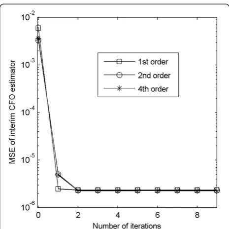
ith interim CFO estimator, respectively. In Figure 1, assuming a small true CFO of δ= 0.18 with a 30-dB signal-to-noise ratio (SNR), we present the learning curves of the MSE of the interim CFO estimator (i.e.,
Var δ^ð Þi
h i
vs. i) for three approximation orders K= 1,
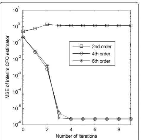
2, and 4. Note that no Gram-Schmidt QR transform-ation is executed for the first-order algorithm. From the figure, we see that the first-order algorithm takes one iteration step or one correction cycle (i= 1) to reach the steady-state value, while the second and fourth algorithms need two correction cycles (i= 2). This may be because the heavy computation load re-quired by higher degree polynomials will encumber the correction process. We have mentioned earlier that when the polynomial degree K is too high, the trian-gularization process will begin to give less accurate results [34]. Then, Figure 2 shows the results of re-peated experiments using a larger δ= 0.48. The result of the sixth-order algorithm is now added. This time,
the first-order algorithm fails to deliver an acceptable re-sult. Again, for the similar reason of computational encumbrance by high-order process, the second-order algorithm has a smoother path to reach the steady state needing two correction iterations (i= 2), while
Figure 1Learning curves of MSE of interim CFO estimator for approximation algorithms of various orders,δ= 0.18, SNR = 30 dB,L= 2.
both the fourth- and sixth-order algorithms require one more iterations (i= 3) and struggle slightly on way to convergence (the learning curves experience small fluctuations). However, if we increaseδfurther beyond half the carrier spacing (|δ| > 0.5), we shall begin to see the advantage of using higher orders. In Figure 3, the curves usingδ= 0.6 are presented. Now, lower order al-gorithms (K≤2) start to diverge. However, the high-order algorithms (fourth and sixth) can still deliver good performance with the higher order (sixth order) doing better.
From Figures 1, 2 and 3, the minimum required correc-tion cycles ensuring convergence for carrier frequency off-sets of 0.18, 0.48, and 0.6 are 2, 3, and 4, respectively, for the proposed method. Accordingly, we choose the correc-tion cycle parameterM= 4 for all the subsequent simula-tions for our proposed method.
Next, over the same channel system with the small fre-quency drift ofδ= 0.18, Figures 4 and 5 respectively give the performance curves of the final CFO estimator MSE (i.e., Varh i^δ or Var δ^ð Þm
h i
) vs. SNR and CIR estimator
MSE Var h^ h i
vs. SNR for various algorithms including
those of the EM-based algorithm and JML-CFE algo-rithm given by [12,14]. For all the estimator MSE per-formance curves, results are averaged over 10,000 runs. Also incorporated in the figure is the Cramer-Rao bound
(CRB) vs. SNR curve for performance comparison. The derivations for CRB are presented in the Appendix for clarity. For this small frequency drift, we see that our al-gorithms of order K= 1, 2, and 4 all yield comparable performance with estimator MSE curves adhering closely
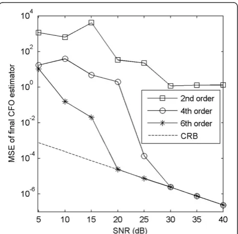
Figure 4MSE of final CFO estimator vs. SNR curves for various algorithms withδ= 0.18.
Figure 5MSE of CIR estimator vs. SNR curves for various algorithms withδ= 0.18.
to the CRB curve, and they all outperform the EM-based and the JML-CFE algorithms. In fact, it can be apparently seen that the EM-based algorithm performance is un-acceptable. Simulation results show that the EM-based algorithm can work well only with δ< 0.05. The reason that the EM-based algorithm works poorly may be due to the fact that the expectation step uses MMSE esti-mate rather than ML estiesti-mate for the CIR in addition to the poor use of low first-order approximation. If we increase δ to 0.48, we will find that all the first-order algorithms including ours will all fail to work, while the three high-order algorithms (K= 2, 4, 6) still perform comparably with estimator MSE curves very closely ad-hering to the CRB (results not shown for space saving). For δ values beyond half the carrier spacing, Figures 6 and 7 respectively plot the curves of final CFO estima-tor MSE and the CIR estimaestima-tor MSE against SNR along with the CRB curves for δ= 0.6. Orders 2, 4, and 6 are given. We can now see that the sixth-order algorithm clearly prevails as both the CFO and CIR estimator MSEs will begin to adhere closely to the CRBs from SNR = 20 dB, while for the fourth-order algorithm, the SNR must be greater than 30 dB for estimator MSEs to closely adhere to the CRBs. For orders K≤2, the algo-rithm will fail to perform atδ= 0.6 just as in Figure 3.
Although the estimator MSE is an important and very useful performance metric for parameter estimations, the ultimate performance measure in communication systems belongs to error rate. We therefore should
compare the error rate performances of various algo-rithms. It is well known that OFDM error rate perform-ance relies on the accuracies of frequency and channel estimation [30]. A good tracking scheme should achieve better CFO and CIR estimations hence lower error rate. Employing 16-ary square QAM transmission over the same channel system, with small frequency driftδ= 0.18, Figure 8 compares SER vs. SNR curves for all the first-order schemes as well as the second-first-order algorithm. Clearly, both the schemes of [12] and [14] fail to per-form satisfactorily, while our first- and second-order algorithms perform comparably well with SER values just slightly higher than an ideal case (perfect CFO synchronization and channel estimation). Then, we as-sume a larger CFO δ= 0.6. Now as shown in Figure 9, both our first- and second-order algorithms fail to work. The fourth- and sixth-order algorithms perform comparably well with SER curve slightly higher than the ideal result.
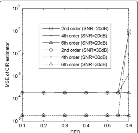
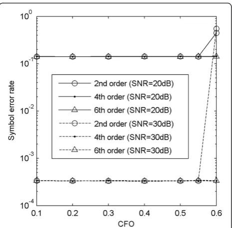
Figures 10 and 11 show the MSE of final CFO estimate vs. CFO δ and the MSE of CIR estimator vs. CFO δ, respectively, at fixed SNR. Both the figures show that the sixth-order algorithm works well for CFO up to 0.6, while the second-order algorithm performs comparably well with the sixth order for CFO up to 0.55 but fails when CFO approaches 0.6. For the fourth order, when the SNR is greater than 30 dB, it performs comparably well with the sixth order. The results show agreement
Figure 7MSE of CIR estimator vs. SNR curves for various algorithms withδ= 0.6.
with what we get from Figures 4, 5, 6 and 7, in which only two specific CFO values, 0.18 and 0.6, are consid-ered. Figure 12 shows the curves of SER vs. CFO δ. It shows agreement with what we get from Figures 8 and 9 that the fourth and the sixth have the comparable
performance in terms of SER up to CFO of 0.6. No-tice that seeing from Figures 4, 5, 6, 7, 10 and 11, the fourth order has poor MSEs for both the CFO and CIR estimators working on CFO approaching 0.6 at low SNR, i.e., SNR = 20 dB. However, seeing from
Figure 9Curves of 16-QAM SER vs. SNR for approximation algorithms of various orders withδ= 0.6.
Figure 8Curves of 16-QAM SER vs. SNR for low-order approximation algorithms withδ= 0.18.
Figure 10MSE of final CFO estimator vs. CFO curves for fixed SNR.
Figures 8, 9 and 12, the SER curves of the fourth order are closely attached to those of the sixth order for CFO up to 0.6 for all values of SNR. This means that, at low SNR which corresponds to high SER, the SER performance makes no difference for the fourth-and sixth-order algorithms even though they have big differences in MSE values at low SNR. Since the ultimate performance depends on SER, instead of MSE, we con-clude that the fourth order will suffice for covering the CFO exceeding half the subcarrier spacing.
By observing various simulation results, we can conclude that, for a tracking range up to |δ| < 0.6, the fourth-order algorithm should suffice. To cover a wider tracking range, one can use orders higher than 4. However, using or-ders higher than 4 is not recommended since it will only increase the computation load without much gain
except for a wider tracking range which is rarely neces-sary for fine frequency tracking. In fact, for fine fre-quency tracking, the frefre-quency drift ought to be less than half the carrier spacing or |δ| < 0.5. The |δ| < 0.5 range is already a much wider range than those covered by all the existing tracking algorithms cited previously. Our second-order algorithm can easily cover this range with adequate performance. Thus, our proposed algo-rithm design indeed provides a significant contribution to the OFDM tracking study.
The significant performance improvement provided by our high-order approximation algorithm is not without price. It is conceivable that the higher the order, the higher is the computation complexity and hence more complicated and costly it will be for practical implementation. Depending on the application, a trade-off between complexity and performance may be made. Table 1 evaluates and compares the computation com-plexities of various algorithms discussed in this paper. It is seen that the complexity of an algorithm is related to channel dispersion length v, OFDM symbol block length
N, order of approximationK, as well as iteration number
M in a rather complicated way. Generally, higher ap-proximation order will give higher complexity. Usually,N
is much larger thanv,K, orM and hence has the domin-ant impact on the computation complexity. Thus, from Table 1, we can get a rough estimate that, among the first-order approximation algorithms, the EM-based algo-rithm should have the lowest complexity, but its per-formance is poorest. Our first-order algorithm may have higher complexity than the EM-based and the JML-CFE algorithms, but not much higher. Therefore, in light of all the gaining in tracking range, estimation accuracy, and error rate performance, it should be well worthwhile to adopt our algorithm.
5. Conclusions
To track frequency drift and channel state variation in OFDM systems over mobile wireless channels, we propose
Figure 12Curves of 16-QAM SER vs. CFO for fixed SNR.
Table 1 Computation complexity comparison between various tracking algorithms
Real multiplication Real addition Real division Square roots
EM (M+ 1)(8vN+ 13N−1) 2(M+ 1)(2vN+N−v−2) M+ 1 0
JML-CFE 2N(13N+ 2v+ 8) 12N2+ 2vN−3N−2v−6 1 0
The first-order algorithm ðMþ1Þ8N2þ13N−1
þ4vN
Mþ1
ð Þ4N2−3
þ2v Nð −1Þ−1 M+ 1 0
TheKth-order algorithm (K≥2)
Mþ1
ð Þð20Kþ8ÞN2
þð5Kþ4ÞN þK L3K2−1−1
þ4vN
Mþ1
ð Þ2 2Kð þ1ÞN2 −2ðKþ1ÞN
þL Kð −1Þ3K2þK=2−1
þMþ2v Nð −1Þ
Mþ1
ð Þ
LKð3K−1Þ=2þK
a high-order approximation algorithm using the MLE scheme which outperforms existing OFDM tracking algo-rithms in terms of tracking range, estimation accuracy, as well as SER performance. Computer simulation results show that a fourth-order algorithm will suffice to cover a wide tracking range exceeding half the carrier spacing while producing results with good accuracy. A second-order algorithm will suffice if the tracking range is less than half the carrier spacing.
Appendix
Cramer-Rao bounds
Define the following real vectors by stacking the real and imaginary parts of corresponding complex vectors as
r¼ Ref gr T;Imf gr T
Then, the log-likelihood function of (7) can be rewrit-ten as
The fisher information matrix for the real vector θ is given by [35] using (A6), we can write
J θ ¼ 2
Now, using the following facts
∂DδFHNXFvh
the Fisher information of (32) can be expressed as
The Cramer-Rao bounds (CRBs) can then be obtained from the diagonal elements of J−1. Note that the CRBs obtained here are jointly for the ML estimates of CIRh and CFOδ(i.e.,h^ and^δ).
Abbreviations
CFO:carrier frequency offset; CFR: channel frequency response; CIR: channel impulse response; DFT: discrete Fourier transform; EM: expectation-maximization; i.i.d: independent, identically distributed; JML-CFE: joint maximum-likelihood channel and frequency estimation; ML: maximum-likelihood; MLE: ML estimation; OFDM: orthogonal frequency division multiplexing; RLS: recursive least squares; RV: random variable; SER: symbol error rate.
Competing interests
The authors declare that they have no competing interests.
Author details
1Department of Electrical Engineering, Tamkang University, No. 151,
Yingzhuan Rd., Danshui Dist, New Taipei City 25137, Taiwan.2Department of Electrical Engineering, Fu Jen Catholic University, No. 510, Zhongzheng Rd., Xinzhuang Dist, New Taipei City 24205, Taiwan.
Received: 18 July 2013 Accepted: 6 January 2014 Published: 27 January 2014
References
1. T Keller, L Piazzo, P Mandarini, L Hanzo, Orthogonal frequency division multiplex synchronization techniques for frequency-selective fading channels. IEEE. J. Seclected Areas Commun.19(6), 999–1008 (2001)
2. PH Moose, A technique for orthogonal frequency division multiplexing frequency offset correction. IEEE Trans. Commun.42(10), 2908–2914 (2001) 3. JJ van de Beek, M Sandell, PO Borjesson, ML estimation of time and frequency
offset in OFDM systems. IEEE. Trans Signal Proces.45(7), 1800–1805 (1997) 4. TM Schmidl, DC Cox, Robust frequency and timing synchronization for
OFDM. IEEE Trans. Commun.45(12), 1613–1621 (1997)
5. YH Kim, JH Lee, Joint maximum likelihood estimation of carrier and sampling frequency offsets for OFDM systems. IEEE Trans. Broadcast.57(2), 277–283 (2011) 6. WL Chin, ML estimation of timing and frequency offsets using distinctive
correlation characteristics of OFDM signals over dispersive fading channels. IEEE. Trans. Vehicular Technol.60(2), 444–456 (2011)
7. YS Choi, PJ Voltz, FA Cassara, ML estimation of carrier frequency offset for multicarrier signals in Rayleigh fading channels. IEEE. Trans. Vehicular Technol.50(2), 644–655 (2001)
8. BB Salberg, A Swami, Doppler and frequency-offset synchronization in wideband OFDM. IEEE. Trans. Wireless Commun.4(6), 2870–2881 (2005) 9. M Morelli, U Mengali, Carrier-frequency estimation for transmissions over
selective channels. IEEE Trans. Commun.48(9), 1580–1589 (2000) 10. X Ma, H Kobayashi, SC Schwartz,Joint frequency offset and channel estimation
for OFDM. Proceedings of the IEEE GLOBECOM 2003, vol. 1(IEEE, Piscataway, San Francisco, 2003), pp. 15–19
11. L Zheng, W Cheng, J Hu, D Yuan,The ML frequency tracking algorithm for OFDM systems based on pilot symbols and decision data. Proceedings of the IEEE International Symposium on Microwave, Antenna, Propagation, and EMC Technologies for Wireless Communications, vol. 2(IEEE, Piscataway, Beijing, 2005), pp. 1611–1614
12. JH Lee, JC Han, SC Kim, Joint carrier frequency synchronization and channel estimation for OFDM systems via the EM algorithm. IEEE. Trans. Vehicular Technol.55(1), 167–172 (2006)
13. MO Pun, M Morelli, CCJ Kuo, Maximum-likelihood synchronization and channel estimation for OFDMA uplink transmissions. IEEE Trans. Commun. 54(4), 726–736 (2006)
14. FZ Merli, GM Vitetta, Iterative ML-based estimation of carrier frequency offset, channel impulse response and data in OFDM transmissions. IEEE Trans. Commun.56(3), 497–506 (2008)
15. JJ van de Beek, O Edfors, M Sandell, SK Wilson, PO Borjesson,On channel estimation in OFDM systems. Proceedings of the IEEE 45th Vehicular Technology Conference(IEEE, Piscataway, Chicago, 1995), pp. 815–819
16. O Edfors, M Sandell, JJ van de Beek, SK Wilson, PO Borjesson, OFDM channel estimation by singular value decomposition. IEEE Trans. Commun. 46(7), 931–939 (1998)
17. Y Li, Pilot-symbol-aided channel estimation for OFDM in wireless systems. IEEE. Trans. Vehicular Technol.49(4), 1207–1215 (2000)
18. Y Li, Simplified channel estimation for OFDM systems with multiple transmit antennas. IEEE. Trans. Wireless Commun.1(1), 67–75 (2002)
19. Y Li, JH Winters, NR Sollenberger, MIMO-OFDM for wireless communications: signal detection with enhanced channel estimation. IEEE Trans. Commun. 50(9), 1471–1477 (2002)
20. S Coleri, M Ergen, A Puri, A Bahai, Channel estimation techniques based on pilot arrangement in OFDM systems. IEEE Trans. Broadcast. 48(3), 223–229 (2002)
21. H Nguyen-Le, T Le-Ngoc, CC Ko, RLS-based joint estimation and tracking of channel response, sampling, and carrier frequency offsets for OFDM. IEEE Trans. Broadcast.55(1), 84–94 (2009)
22. M Jamalabdollahi, S Salari, B Zahedi,Efficient joint frequency synchronization and channel estimation in OFDM systems. Proceedings of the IEEE 19th Conference on Signal Processing and Communications Applications(IEEE, Piscataway, Antalya, 2011), pp. 206–209
23. Y Liu, Z Tan, H Wang, KS Kwak, Joint estimation of channel impulse response and carrier frequency offset for OFDM Systems. IEEE. Trans. Vehicular Technol.60(9), 4645–4650 (2011)
24. S Salari, RS Kandovan,Joint frequency and channel estimation for MIMO-OFDM systems via the EM algorithm. Proceedings of the IEEE Wireless and Optical Communications Networks(IEEE, Piscataway, Colombo, 2010), pp. 1–5 25. EP Simon, L Ros, H Hijazi, M Ghogho, Joint carrier frequency offset and
channel estimation for OFDM systems via the EM algorithm in the presence of very high mobility. IEEE. Trans. Signal Proces.60(2), 754–765 (2012) 26. G Sewell,Computational Methods of Linear Algebra, 2nd edn. (Wiley, New
York, 2005)
27. GH Golub, CF Van Loan,Matrix Computations, 3rd edn. (The Johns Hopkins University Press, Maryland, 1996)
28. JFG Francis, The QR transformation, a unitary analogue to the LR transformation-part 1. Comp. J.4(3), 265–271 (1961)
29. JG Proakis, M Salehi,Digital Communications, 5th edn. (McGraw-Hill, New York, 2008)
30. RY Yen, HY Liu, WK Tsai, QAM symbol error rate in OFDM systems over frequency-selective fast Ricean fading channels. IEEE. Trans. Vehicular Technol. 57(2), 1322–1325 (2008)
31. M Morelli, CJ Kuo, MO Pun, Synchronization techniques for orthogonal frequency division multiple access (OFDMA): a tutorial review. Proc. IEEE 95(7), 1394–1427 (2007)
32. P Stoica, O Besson, Training sequence design for frequency offset and frequency-selective channel estimation. IEEE Trans. Commun. 51(11), 1910–1917 (2003)
33. DC Chu, Polyphase codes with good periodic correlation properties. IEEE. Trans. Info. Theory.18(4), 531–532 (1972)
34. S Haykin,Adaptive Filter Theory, 4th edn. (Prentice Hall, New Jersey, 2002) 35. SM Kay,Fundamentals of Statistical Signal Processing, Volume I: Estimation
Theory(Prentice Hall, New Jersey, 1993)
doi:10.1186/1687-1499-2014-16
Cite this article as:Yenet al.:High-order approximation algorithm using