Analysis of dynamics in an eco epidemiological model with stage structure

(1)

R E S E A R C H

Open Access

Analysis of dynamics in an

eco-epidemiological model with stage

structure

Pengmiao Hao, Junjie Wei

*

_{and Dejun Fan}

*_{Correspondence: [email protected]} Department of Mathematics, Harbin Institute of Technology, Harbin, Heilongjiang 150001, P.R. China

Abstract

This paper is devoted to the study of an eco-epidemiological model with stage structure in the predator and disease in the prey. To begin with, the positivity and boundedness of the solutions are obtained. This shows that the system possesses a bounded absorbing set. Then, by using the LaSalle-Lyapunov invariance principle, limit equation theory, and a geometrical criterion for analyzing the distribution of the eigenvalues, the stability of the boundary equilibria and interior equilibrium are established, respectively. Meanwhile, the existence of Hopf bifurcations is obtained when the delay

τ

varies in a limitary region. Furthermore, by employing center manifold theory and the normal form method, an algorithm for determining the direction and stability of the Hopf bifurcation is derived. At last, some numerical simulations are carried out for illustrating the analytic results.

Keywords: eco-epidemiological model; time delay; stage structure; stability; Hopf bifurcation

1 Introduction

Ecological models that reveal the amounts of prey and predator have long been and still will be investigated for their universal existence and importance. After the fundamental work of Lotka and Volterra for prey interactions in the middle of s, predator-prey models were studied extensively [–]. Some literature considered the stage struc-ture, assuming the immature predator does not consume the prey. Suppose the constant death rate of the immature predator to bed, then the livability ise–dt_after_t_{time passed.} An epidemiological model is also widely studied. The most frequent types are SI, SIS, SIR, and SIRS. As is well known, the basic reproduction numberRmakes a signiﬁcant role

in such model. It presents the average number of new susceptible cells acquired from a single infected cell, and determines the persistence of the disease.

The so-called eco-epidemiological model is the combination of infection into ecolog-ical model. It contains two types mainly: disease in the predator [] and disease in the prey [–, , ]. When we have disease in the prey, the predator may consume on both the healthy and infected prey [, ]. Sometimes the infected ones are weaker or say, their habitats are accessible to the predator (e.g.infected ﬁsh stay close to the water surface and thus are easy to capture). The literature shows that the predation rate on infected prey

(2)

may be  times higher than on susceptible prey []. Thus sometimes it is reasonable to

say that the predators consume the infected prey only []. The pioneer work for study of

eco-epidemiological model is Anderson and May [] in . After that, Chattopadhyay

and Arino [] used the name ‘epidemiological’ ﬁrst. For the detailed evolution of

eco-epidemiological model we refer to Bairagi and Chattopadhyay [].

Usually, an eco-epidemiological model of SI type contains three variables: the suscepti-ble preyS(t), infected preyI(t), and predatorP(t). We have the following assumptions:

• Only susceptible prey are capable to reproduce under the logistic law with intrinsic

birth rate constantr> and carrying capacityK> , while the infected prey also

contribute to the carrying capacity.

• The bilinear incidence with rateξmake the disease spreads from infected to

susceptible prey.

• Suppose the infected prey are vulnerable, thus easier to catch, so the predation on

susceptible prey is ignored. The predation on infected prey follows a Holling type II

response function.

• The natural death rates of infected prey and predator areμandd, respectively.

Assumedto be death rate of predator due to consuming of infected prey, so the total

death rate of predator isd=d+d. Furthermore, assume the predator has no food

source other than infected prey, and the toxicity level is taken to be low enough that

eating infected prey does more good than harm.

Chattopadhyay and Bairagi [] have proposed an eco-epidemiological model in the

fol-lowing form:

˙ S=rS

 –S+I K

–ξIS,

˙

I=ξIS– mIP a+I–μI,

˙

P=mαIP a+I –dP.

(.)

The local and global stability of the system (.) around the biologically feasible equilibria

is obtained in [].

It is realistic and interesting for us to construct the stage-structured eco-epidemiological

model and study the combined eﬀects of stage structure and mutual interference by

preda-tors. On the meaning of the construction of a stage-structured eco-epidemiological model

we refer to Liu and Beretta []. Most existing stage-structure models (see [–] and the

references therein) deal with single species growth, which assumes a constant resource

supply []. Gourley and Kuang [] formulated a robust stage-structured predator-prey

model with the assumption that stage-structured consumer species growth is a combined

result of birth and death processes, both of which are closely linked to the dynamical

(3)

we formulate the robust stage-structured eco-epidemiological model as follows:

˙

S(t) =rS(t)

 –S(t) +I(t) K

–ξI(t)S(t),

˙

I(t) =ξI(t)S(t) –mI(t)P(t) a+I(t) –μI(t),

˙

p(t) =mαI(t)P(t) a+I(t) –

mαI(t–τ)P(t–τ) a+I(t–τ) e

–dτ_–_d

p(t),

˙

P(t) =mαI(t–τ)P(t–τ) a+I(t–τ) e

–dτ_–_dP(t),

(.)

where S(t) andI(t) are as mentioned above,p(t) andP(t) represent the immature and mature predator densities, respectively. We assume that the immature predators suﬀer a mortality rate ofd(the through-stage death rate) and takeτunits of time to mature; thus

e–dτ _{is the surviving rate of each immature predator to reach maturity.}

Notice that the ﬁrst, second, and fourth equations of system (.) are independent of the variablep(t), we see that (S(t),I(t),P(t)) satisfy the following system:

˙

S(t) =rS(t)

 –S(t) +I(t) K

–ξI(t)S(t),

˙

I(t) =ξI(t)S(t) –mI(t)P(t) a+I(t) –μI(t),

˙

P(t) =mαI(t–τ)P(t–τ) a+I(t–τ) e

–dτ

–dP(t).

(.)

The purpose of the paper is to study the dynamics of (.). The rest of this paper is organized as follows: In Section , the properties of the solutions such as positivity and boundedness are obtained. In Section . the stability of the boundary equilibria are spec-iﬁed by using an eigenvalue analysis and the LaSalle-Lyapunov method. The existence and properties of a Hopf bifurcation are investigated in Sections . and ., respectively. Fi-nally, some simulations are carried out for illustrating the analytic results in Section .

2 Positivity and boundedness

In this section, we shall investigate the positivity and boundedness of the solutions of sys-tem (.) with nonnegative initial conditions. DeﬁneC=C([–τ, ],R), thenCis a Banach space under the norm

|ϕ|= sup θ∈[–τ,]

ϕ(θ).

Hence,R×C×Ccan be regarding as a phase space of system (.). In the following, we consider system (.) with nonnegative initial condition:

ϕi(θ)≥ on –τ≤θ≤ (i= , , ), (.)

whereϕ(θ)≡const∈R. We have the following conclusion.

(4)

Proof Let (S(t),I(t),P(t)) be the solution of (.) with initial condition (.). Then from the ﬁrst and second equation in (.) we have

S(t) =ϕ()e t

[r(–S(σ)+KI(σ))–ξI(σ)] dσ

and

I(t) =ϕ()e t

[ξS(σ)–amP+I(σ)(σ)–μ] dσ_,

respectively. These show thatS(t)≥ andI(t)≥ for allt≥. Particularly,S(t) >  when

ϕ() > , andI(t) >  whenϕ() > , for all t≥. AndS(t)≡ when ϕ() = , and

I(t)≡ whenϕ() = .

Next we show thatP(t)≥. From the third equation in (.) we have

˙

P=mαϕ(t–τ)ϕ(t–τ) a+ϕ(t–τ)

e–dτ_–_dP, _for_t∈_[,_τ_].

Then byϕandϕbeing both nonnegative, it follows thatP˙≥–dP. This implies that

P(t)≥ϕ()e–dt≥ fort∈[,τ].

Fort∈[τ, τ], from the third equation in (.) and the discussion above, we have

˙

P=mαI(t–τ)P(t–τ) a+I(t–τ) e

–dτ_–_dP≥_–dP.

This implies that

P(t)≥P(τ)e–d(t–τ)≥ fort∈[τ, τ].

By mathematical induction, one can obtain P(t)≥ for any positive integernandt∈ [nτ, (n+ )τ]. Hence we haveP(t)≥ for allt≥.

We choose the following function:

y(t) =S(t) +I(t) +e dτ

α P(t+τ),

to consider the boundedness of positive solutions. Calculating the derivative ofy(t) along the solution of system (.), we get

˙ y(t) =rS

 –S+I K

–μI–de dτ

α P(t+τ).

Then there exists a positive constantδ(δ≤min(μ,d)), such that

˙

y+δy≤(r+δ)S– r KS

_.

Then we obtain

˙

(5)

wherec=K(r_+_rδ). Thuslimt→∞y(t)≤ cδ. This implies that, for any nonnegative solution

(S(t),I(t),P(t)), of (.), there exists aT≥τsuch that

S(t) +I(t) +e dτ

α P(t+τ) <c+ε, t>T,

whereεis some positive number. Hence, the nonnegative solutions of system (.) is

uni-formly eventually bounded.

Remark . From the proof above, we have|Pt|<αe–dτ(c+ε) whent>T+τ.

Lemma . For system(.)with initial condition(.),if|ϕ+ϕ|<K,then

S(t) +I(t) <K for t≥.

In fact, from the ﬁrst and second equations in (.) we have

d

dt(S+I) =rS

 –S+I K

– mIP

a+I –μI. (.)

In the case ofϕ() = , by the expression ofI(t) we know thatI(t)≡. Hence (.)

be-comes

dS dt =rS

 – S K

.

This implies thatS(t) <Kwhenϕ<K, that is,S(t) +I(t) <Kfort≥.

In the case ofϕ() > , by the expression ofI(t) we know thatI(t) >  fort≥. For a

contradiction, we assume that there exists at>  such that

S(t) +I(t)≤K fort∈[,t),

andS(t) +I(t) =K. Then it follows that

d dt(S+I)

t=t

= –mI(t)P(t) a+I(t)

–μI(t) < .

The contradiction implies that the conclusion follows. LetR+= [,∞) andC+=C([–τ, ],R+). Deﬁne

=

(ϕ,ϕ,ϕ)∈R+×C+×C+:|ϕ+ϕ|<K,|ϕ|<

c

δ+ε

αe–dτ

,

wherecandδare in the denotation of the previous proof,εis arbitrarily small positive number.

By Theorem . and Lemma . we know that all solutions eventually enter and remain in the region. This means that, for (.),is a bounded absorbing set.

3 Stability and existence of Hopf bifurcation

(6)

3.1 Boundary equilibria and their stability

Clearly, system (.) always has two nonnegative equilibria given by

E: (, , ) and E: (K, , ).

And when

R:=

Kξ

μ >  (.)

is satisﬁed, another boundary equilibrium is given by

E: (S,I, ) =

μ ξ,

r(Kξ–μ)

ξ(r+Kξ), 

.

Moreover, we make the following assumption:

mαe–dτ

–d>  (.)

throughout this paper, and when

R:=

Kξ μ –

adξ(Kξ+r)

rμ(mαe–dτ _–_d)>  (.)

is satisﬁed, system (.) has a unique positive equilibrium given by

E∗:=S∗,I∗,P∗

=

K– ad(Kξ+r) r(mαe–dτ _–_d),

ad mαe–dτ_–_d,

 m

a+I∗ ξS∗–μ . (.)

In fact, (.) is equivalent to

K– ad(Kξ+r) r(mαe–dτ_–_d)>

μ ξ,

henceS∗> , andP∗> .

Clearly,R>R. AndR is the basic reproduction number of infection for (.) with τ = . On the deﬁnition of the basic reproduction number of infection, we refer to []. In the following, we use the notations introduced in []. Then system (.) withτ=  is rewritten in the following form:

˙

I=ξIS– mIP a+I–μI,

˙ S=rS

 –S+I K

–ξIS,

˙

(7)

Figure 1 Regions of equilibria existence in (R0,

R1) plane.

Then the infected compartment isIwithm=  andn= . Meanwhile,

F =

⎛ ⎜ ⎝

ξIS  

⎞ ⎟ ⎠

and

V =

⎛ ⎜ ⎝

mIP a+I +μI

ξIS–rS( –S+I K ) dP–m_aα₊IP_I

⎞ ⎟ ⎠.

The equilibrium solution withI=  isE(,K, ). Following the description in [] we have

F=

∂F

∂I

(,K,)

=ξS|(,K,)=Kξ,

V=

∂V

∂I

(,K,)

= amP

(a+I) +μ

(,K,)

=μ.

Thus the basic reproduction number of infection isR=ρ(FV–) =Kμξ.

Deﬁne

τ=  d

ln mα

d+ad_r₍ξ_K(K_ξ_–ξ_μ+₎r). (.)

Then from the discussion above we know that, under the assumption (.), system (.) has a positive equilibrium when ≤τ<τ_.

We can see that the value ofRandRare signiﬁcant to the existence of equilibria, for

intuit, we divide the_ plane (R>R> ) of existence regions for the equilibria into three

parts as in Figure .

In this ﬁgure, the oblique line denotesR=R. When  <R<R< ,EandE exist;

when  <R<  <R,E,E, andEexist; when  <R<R,E,E,E, andE∗exist. In the

following we study the stability of the nonnegative equilibria.

Theorem . For system(.),the following statements are true.

(i) Eis always unstable.

(8)

Proof (i) The linearization of (.) at the originEis given by

˙ S=rS,

˙ I= –μI,

˙ P= –dP.

Its characteristic equation is

(λ–r)(λ+μ)(λ+d) = .

Notice thatλ=r> , thenEis unstable.

(ii) The linearization of (.) at the ﬁxed pointE= (K, , ) is given by

˙

S= –rS– (r+Kξ)I,

˙

I= (ξK–μ)I,

˙ P= –dP,

whose characteristic equation is

(λ+r)λ– (Kξ–μ) (λ+d) = .

We can seeλ,< , and

λ=Kξ–μ

< , whenR< ,

> , whenR> .

Hence,Eis asymptotically stable whenR<  and unstable whenR> .

We choose a Lyapunov functionalL:R×C×C→Ras L(ϕ,ϕ,ϕ) =ϕ().

The derivative ofLalong the solutions of system (.) is

L|()=I(t) =ξIS–

mIP a+I –μI ≤I(ξK–μ)

=μI(R– ).

Therefore,L|()≤ for allS,I,P≥ whenR< , andL =  if and only ifI(t) = . That is,

S=ϕ∈:L(ϕ) = =(ϕ, ,ϕ)

.

Deﬁne

M:=E,E, (R+, ,R+)

(9)

ThenMis the maximal invariant set under (.) inS. In fact, substitutionI=  into (.) leads to the following initial value problem:

˙ S=rS

 – S K

,

˙ P= –dP,

S(t) =ϕ(t) > , P(t) =ϕ(t) > , –τ≤t≤.

(.)

The claim follows. Clearly,

lim

t→∞S(t) =K, tlim→∞P(t) = .

By Theorem . in [], Chapter , we know that any solution (St,It,Pt) of (.) with initial valueϕ∈ ¯tends toMast→ ∞. Notice the structure ofM, we have

lim

t→∞It= .

Hence, from the third equation in (.) it follows that

lim

t→∞Pt= .

Now we consider the ﬁrst equation in (.),

˙ S=rS

 – S K

–

ξ+ r

K

IS (.)

and

˙ y=ry

 – y K

. (.)

Let

f(t,S) =rS

 – S K

–

ξ+ r

K

I(t)S and g(y) =ry

 – y K

.

Then fromlimt→∞I(t) =  we have

f(t,S)→g(S), t→ ∞, locally uniformly inS∈R.

We know that{K}is an asymptotically stable equilibrium of (.). It is well known that for anyS> , the solutionSof (.) with initial valueS>  is bounded fort≥. Denote the ω-limit set of the forward bounded solution of (.) asω(,S). Then for anyy∈ω(,S),

we see that the solution of (.) withy() =y>  converges toK ast→ ∞. Applying

Theorem . in [] it follows thatS(t)→K ast→ ∞. ThusEis globally attractive in whenR< . Furthermore, combined with the local stability ofEit implies that it is

(10)

(iii) The linearization of (.) at the ﬁxed pointE= (μξ,

we will turn to the study of

λ=

3.2 Interior equilibrium and its stability

In this subsection, we always assumeR> , and we will concentrate on the study of the

interior equilibriumE∗(S∗,I∗,P∗). Let

˜

S=S–S∗, ˜I=I–I∗, P˜=P–P∗. (.)

Then the interior equilibriumE∗(S∗,I∗,P∗) of system (.) is moved to the origin. We re-move the superscript for the sake of convenience. Then (.) becomes

(11)

dP

Obviously, the origin (, , ) is an equilibrium of system (.). Denote

B(τ) =

So the linearization of (.) at the origin is given by

⎛

(12)

(a+b)(a+b) – (a+b)

By the Hurwitz criterion, we make the following assumptions on (.):

(H) : a() +b() > ,

(H) : a() +b() > ,

(H) : a() +b() a() +b() –

a() +b() > ,

under which we have the following theorem.

Theorem . Assume R> and(H)-(H)are satisﬁed.Then the positive equilibrium E∗

of (.)is asymptotically stable whenτ= .

(13)

In order to investigate the purely imaginary roots of (.) by using the method intro-duced by Beretta and Kuang [], we rewrite equation (.) as

P(λ,τ) +Q(λ,τ)e–λτ= ,

with

P(λ,τ) =λ+aλ+aλ+a, Q(λ,τ) =bλ+bλ+b. (.)

Before applying the geometry criterion in [] to (.), a sequence of conditions onPand Qare required to be veriﬁed. This is accomplished by the following proposition.

Proposition . Letτ₌ 

dln

mα

(+K_rξ)ad/(K–μ_ξ)+d,and P and Q are deﬁned in(.).Then the following statements are valid for allτ ∈[,τ_).

(a) P(,τ) +Q(,τ)= ; (b) P(iω,τ) +Q(iω,τ)= ;

(c) lim{|Q_P(₍_λλ,_,_ττ)₎|:|λ| → ∞,Reλ≥}< for anyτ;

(d) F(ω,τ) :=|P(iω,τ)|–|Q(iω,τ)|has a ﬁnite number of real zeros for eachτ; (e) each positive rootω(τ)ofF(ω,τ) = is continuous and diﬀerentiable inτ whenever

it exists.

Proof

(a) P(,τ) +Q(,τ) =a+b> , that is,λ= is not a root of (.). (b) By the assumption (H), we know that (b) is true.

(c) From

lim

|λ|→∞

Q(_P(_λλ_,,_ττ₎)= lim

|λ|→∞

bλ+bλ+b λ₊_a

λ+aλ+a = ,

we have

lim

|λ|→∞,Reλ≥ Q(λ,τ)

P(λ,τ)

< .

(d) We have

F(ω,τ) =P(iω,τ)–Q(iω,τ)

=ω+a_– a–b ω+

a_– aa–b+ bb ω+

a_–b_ .

It is obvious that property (d) is satisﬁed.

(e) The conclusion is valid becauseF(ω,τ)is a cubic polynomial inω_{and the fact that}

ai(i= , , ) andbj(j= , ) are all continuous functions ofτ.

We also mention that

(14)

P,Qhave real coeﬃcients. This ensures that ifλ=iω, for some realω, is a root of (.), thenλ= –iωis a root of (.) as well. Letλ=iω(ω> ) be a purely imaginary root of equation (.), then

–iω–aω+iaω+a+

–bω+ibω+b (cosωτ–isinωτ) = .

Separating the real and imaginary parts yields

ω–aω=

bω–b sinωτ+bωcosωτ,

aω–a=bωsinωτ–

bω–b cosωτ.

(.)

Squaring both sides of (.) and summing the two equations, we obtain

hω,τ =F(ω,τ) =ω+pω+qω+s= , (.)

wherep=a

– a–b,q=a– aa+ bb–b,s=a–b.

Setz=ω. Then (.) becomes

h(z,τ) =z+pz+qz+s. (.)

Therefore, equation (.) has a pair of purely imaginary roots±iω(τ∗) whenτ=τ∗if and only ifω(τ∗) is the positive root of (.), or equivalently,z∗=ω(τ∗) is the positive root of (.). As follows from (.) we get

sinωτ=bω

_{+ (a}

b–b–ab)ω+ (ab–ab)ω

b

ω+ (bω–b)

,

cosωτ=(b–ab)ω

_{+ (a}

b+ab–ab)ω–ab

b

ω+ (bω–b)

.

(.)

By the deﬁnitions ofP(λ,τ) andQ(λ,τ) as in (.), and applying the property (b) in Propo-sition ., (.) can be written as

sinωτ=Im

P(iω,τ) Q(iω,τ)

,

cosωτ= –Re

P(iω,τ) Q(iω,τ)

,

which yields

P(iω,τ)=Q(iω,τ),

that is,

F(ω,τ) = .

Deﬁne

(15)

andτ₌_sup

τi∈Iτi. Also deﬁneθ(τ)∈[, π] by

sinθ(τ) =bω

_{+ (a}

b–b–ab)ω+ (ab–ab)ω

b_ω_{+ (b}

ω–b)

,

cosθ(τ) =(b–ab)ω

_{+ (a}

b+ab–ab)ω–ab

b_ω_{+ (b}

ω–b)

.

Then we haveω(τ)τ =θ(τ) + nπ obviously. Therefore,iω∗,ω∗=ω(τ∗) > , is a purely imaginary root of (.) if and only ifτ∗is a zero of the functionSn(τ), which is deﬁned by

Sn(τ) =τ–

θ(τ) + nπ

ω(τ) , τ∈I,n∈N. (.)

We also know thatθ(τ)= , π onI in terms of (b) in Proposition ., andSn(τ) are continuous and diﬀerentiable onIfrom Lemma . in []. The following theorem in [] can be used to verify the occurrence of Hopf bifurcations whenτ=τ∗.

Theorem . Assume that Sn(τ) = has a positive rootτ∗∈I for some n∈N.Then there exists a pair of simple purely imaginary roots±iω(τ∗)of (.)atτ=τ∗,and we denote

δτ∗ =Sign

dReλ(τ) dτ

λ=iω(τ∗)

=Sign

∂F

∂ω

ωτ∗ ,τ∗ ×Sign

dSn(τ) dτ

τ=τ∗

, (.)

which determines the direction in which the pair of purely imaginary roots cross the imag-inary axis:from left to right ifδ(τ∗) > ,and from right to left ifδ(τ∗) < .

Proposition . For Sn(τ)deﬁned on[,τ₎_in_{(.),}_{the following properties hold:} (i) Sn() < ,limτ→τSn(τ) = –∞;

(ii) Sn(τ) >Sn+(τ).

Proof By the deﬁnition ofω(τ) andθ(τ), we knowω(τ) > ,θ(τ)∈(, π).

(i) Sn() = –θ()+_ω_()nπ < obviously. Whenτ →τ, we haveω(τ)→andθ(τ)→πby the facts thatsinθ(τ)→andcosθ(τ)→–. Therefore, by (.) we get

lim_τ_→_τS_n(τ) = –∞.

(ii) Sn(τ) –Sn+(τ) =ω(πτ)> due to the positivity ofω(τ).

Remark . IfS(τ) has no zeros inI, then so doesSn(τ), from the degression ofSn(τ)

w.r.t.nfor alln∈N.

Deﬁne the set of possible Hopf bifurcation values by

J=τ∈,τ |Sn(τ) = ,n∈N,

(16)

Theorem . Assume(H)-(H)are satisﬁed for system(.).Then the following

conclu-sions hold:

(i) IfIis empty orS(τ)has no positive zeros in(,τ)whenIis non-empty,which

implies setJis empty,then equation(.)has no pair of purely imaginary roots,

thus the positive equilibriumE∗is asymptotically stable for allτ∈[,τ). (ii) IfJ=∅andδ(τ∗)=  forτ∗∈J,then()undergoes a Hopf bifurcation atE∗when

τ=τ∗.At this time,E∗is asymptotically stable forτ∈[,τmin)∪(τmax,τ).

3.3 Direction and stability of Hopf bifurcation

In the previous section, we can see that a Hopf bifurcation atE∗whenτ passes through certain critical values may happen indeed, and suﬃcient conditions are obtained as well. In this section, we shall study the direction, stability, and the period of the bifurcating periodic solution. The way to do this is the combination of the normal form method and center manifold theory in []. Without loss of generality, letτ∗be any critical value such that equation (.) has a pair of purely imaginary roots±iω∗, and system (.) undergoes a Hopf bifurcation atE∗. Then, by settingτ=τ∗+μ, andμ=  is the Hopf bifurcation value of (.).

After translation (.) and time scalingt→(t/τ), system (.) can be written as

⎛ nents are bounded variation functions forθ∈[–, ], such that

Lμ(φ) = 

–

(17)

In fact,η(θ,μ) can be chosen as

η(θ,μ) =

⎧ ⎪ ⎨ ⎪ ⎩

(τ∗+μ)B(τ∗+μ), θ= ,

, θ∈(–, ),

–(τ∗+μ)B(τ∗+μ), θ= –.

Deﬁne the operatorsA(μ) andR(μ) as

A(μ)φ(θ) =

dφ(θ)

dθ , θ∈[–, ),



–dη(ξ,μ)φ(ξ), θ= ,

(.)

and

R(μ)φ(θ) =

, θ∈[–, ),

G(μ,φ), θ= .

Then system (.) is equivalent to the following operator equation:

˙

Xt=A(μ)Xt+R(μ)Xt,

whereX(t) = (S(t),I(t),P(t))T_and_X

t(θ) =X(t+θ) forθ∈[–, ]. LetC∗:=C([, ], (R₎∗_{). For}_ψ_∈_C∗_{, deﬁne an operator}

A∗ψ(s) =

–dψ_d_s(s), s∈(, ],



–dη(ξ, )ψ(–ξ), s= ,

(.)

and a bilinear inner form

ψ(s),φ(θ)=ψ()φ() –



– θ

ξ=

ψ(ξ–θ) dη(θ)φ(ξ) dξ, (.)

whereη(θ) =η(θ, ). ThenA() andA∗are adjoint operators.

As shown in Section ., we know that±iω∗τ∗are eigenvalues ofA(), thus, they are also eigenvalues ofA∗. It can be veriﬁed that the vectors

q(θ) = (,q,q)Teiω ∗_τ∗_θ

, θ∈[–, ],

and

q∗(s) =  D

,q∗_,q∗_ eiω∗τ∗s, s∈[, ],

are the eigenvectors ofA() andA∗corresponding to the eigenvaluesiω∗τ∗and –iω∗τ∗, respectively, where

q= –

iω∗τ∗K+rS∗

(Kξ+r)S∗ , q= –

amαP∗e–dτ∗_(i_ω∗_τ∗_K₊_rS∗₎

(a+I∗)_[(i_ω∗_τ∗₊_d)eiω∗τ∗_–_d](K_ξ₊_r)S∗, (.)

q∗_= rS∗

K –iω∗τ∗

ξI∗ , q

∗

=

dedτ∗₍rS∗

K –iω∗τ∗)

(18)

and

One can ﬁnd that

q∗(s),q(θ)= .

Following the algorithms provided in [] and using a computation process similar to that in [, , ], we obtain the following coeﬃcients:

(19)

and

which determine the properties of bifurcating periodic solutions. From the discussion in Sections . and ., we have the following results immediately.

Assume that the conditions in (ii) of Theorem . hold. Thenμ,β,T determine the

direction, stability, and period of the corresponding Hopf bifurcation, respectively:

(i) The direction of the Hopf bifurcation of the system (.) at theE∗whenτ=τ∗is

backward (forward) ifμ< (μ> ), that is, there exists a bifurcating periodic solution forτ<τ∗(τ>τ∗) in a suﬃciently smallτ∗-neighborhood;

(ii) The bifurcating periodic solution on the center manifold is unstable (stable) if

β> (β< ); Particularly, the stability of the bifurcating periodic solutions of

(.) is the same as that of bifurcating periodic solutions on the center manifold whenτ∗=τminandτ∗=τmax.

(20)

4 Numerical simulations

Under the guidance of Section ., we choose a set of parameters which satisfy conditions (H)-(H):

r= , K= , ξ= ., m= ., a= ,

μ= ., α= ., d= ., d = ..

(.)

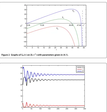
By direct calculation, we haveτ_≈_{. and}_τ_≈_{.. The intersections of}_Sn_with τ-axis imply four Hopf bifurcation points (see Figure ), denoted by

τ≈., τ≈., τ≈., and τ≈..

From Theorem ., we know that the positive ﬁxed point E∗ is asymptotically stable whenτ∈[,τ)∪(τ,τ) (see Figures  and ) and unstable whenτ ∈(τ,τ) (see Figure ).

From the formula (.) and the algorithm derived in Section , we calculate some im-portant quantities as in Table .

It shows us that for system (.) with the data (.):

Figure 2 Graphs ofSn(τ) on [0,τ1_{) with parameters given in (4.1).}

(21)

Figure 4 E∗≈(18.41, 4.85, 24.44) is asymptotically stable whenτ∈(τ4,τ0_{), where} 47.64≈τ4<τ= 48.2 <τ0_≈_{79.978, and the initial condition is (30, 5, 30).}

Figure 5 E∗≈(23.59, 1.93, 28.46) is unstable, and sustained oscillation occurs whenτ∈(τ1,τ4), where 0.58≈τ1<τ= 10 <τ4≈47.64 and the initial condition is (20, 4, 35).

Table 1 List of quantities under (4.1)

∂F

∂ω δ Re(c1(0)) μ2 β2

τ1≈0.58 25.2805 > 0 > 0 –0.8258 < 0 > 0 < 0

τ2≈13.06 18.7185 > 0 > 0 –0.0921 < 0 > 0 < 0

τ3≈39.59 6.1430 > 0 < 0 –0.0230 < 0 < 0 < 0

τ4≈47.64 2.4689 > 0 < 0 –0.0093 < 0 < 0 < 0

. The direction of the Hopf bifurcation at theE∗is forward whenτ=τandτ=τ, and backward whenτ=τandτ=τ, respectively.

. All the bifurcating periodic solutions on the center manifold are stable. Particularly, the bifurcating periodic solutions are stable fromτandτ, respectively.

(22)

Figure 6 Hopf bifurcaton branches starting fromτ1≈0.58,τ2≈13.06 andτ3≈39.59 on the (τ, d) plane, whered= maxS(t) – minS(t).

solution starting fromτ≈. also goes on a long way, and the strange behavior from τ ≈. in the ﬁrst branch needs to be studied.

Competing interests

The authors declare that they have no competing interests.

Authors’ contributions

All authors contributed equally to the writing of this paper. All authors read and approved the ﬁnal manuscript.

Acknowledgements

This research is supported by National Natural Science Foundation of China (No. 11371111), Research Fund for the Doctoral Program of Higher Education of China (No. 20122302110044).

Received: 25 April 2016 Accepted: 24 August 2016 References

1. Qu, Y, Wei, J: Bifurcation analysis in a time-delay model for prey-predator growth with stage-structure. Nonlinear Dyn. 49, 285-294 (2007)

2. Mao, S, Xu, R, Li, Z, Li, Y: Global stability of an eco-epidemiological model with time delay and saturation incidence. Discrete Dyn. Nat. Soc.2011, 730783 (2011)

3. Mukhopadhyay, B, Bhattacharyya, R: Role of predator switching in an eco-epidemiological model with disease in the prey. Ecol. Model.220(7), 931-939 (2009)

4. Chattopadhyay, J, Arino, O: A predator-prey model with disease in the prey. Nonlinear Anal.36(6), 747-766 (1999) 5. Pal, AK, Samanta, GP: Stability analysis of an eco-epidemiological model incorporating a prey refuge. Nonlinear Anal.,

Model. Control15(4), 473-491 (2010)

6. Lafferty, KD, Morris, AK: Altered behavior of parasitized killifish increases susceptibility to predation by bird final hosts. Ecology77(5), 1390-1397 (1996)

7. Anderson, RM, May, RM: The invasion, persistence and spread of infectious diseases within animal and plant communities. Philos. Trans. R. Soc. Lond. B, Biol. Sci.314, 533-570 (1986)

8. Bairagi, N, Chattopadhyay, J: The evolution on eco-epidemiological systems theory and evidence. J. Phys. Conf. Ser. 96, 012205 (2008)

9. Chattopadhyay, J, Bairagi, N: Pelicans at risk in Salton sea - an eco-epidemiological model. Ecol. Model.136, 103-112 (2001)

10. Xiao, Y, Chen, L: A ratio-dependent predator-prey model with disease in the prey. Appl. Math. Comput.131, 397-414 (2002)

11. Liu, S, Beretta, E: A stage-structured predator-prey model of Beddington-DeAngelis type. SIAM J. Appl. Math.66(4), 1101-1129 (2006)

12. Aiello, WG, Freedman, HI: A time-delay model of single-species growth with stage structure. Math. Biosci.101, 139-153 (1990)

13. Liu, S, Chen, L, Luo, G, Jiang, Y: Asymptotic behaviors of competitive Lotka-Volterra system with stage structure. J. Math. Anal. Appl.271, 124-138 (2002)

14. Liu, S, Chen, L, Agarwal, R: Recent progress on stage-structured population dynamics. Math. Comput. Model.36, 1319-1360 (2002)

15. Liu, S, Chen, L, Luo, G: Extinction and permanence in competitive stage structured system with time-delays. Nonlinear Anal.51, 1347-1361 (2002)

(23)

17. Van den Driessche, P, Watmough, J: Reproduction numbers and sub-threshold endemic equilibria for compartmental models of disease transmission. Math. Biosci.180, 29-48 (2002)

18. Hale, J: Theory of Functional Diﬀerential Equations. Springer, New York (1977)

19. Thieme, HR: Convergence results and a Poincaré-Bendixson trichotomy for asymptotically autonomous diﬀerential equations. J. Math. Biol.30(7), 755-763 (1992)

20. Ruan, S, Wei, J: On the zeros of transcendental functions with applications to stability of delay diﬀerential equations with two delays. Dyn. Contin. Discrete Impuls. Syst.10(6), 863-874 (2003)

21. Beretta, E, Kuang, Y: Geometric stability switch criteria in delay diﬀerential systems with delay dependent parameters. SIAM J. Math. Anal.33(5), 1144-1165 (2002)

22. Hassard, BD, Kazarinoﬀ, ND, Wan, YH: Theory and Applications of Hopf Bifurcation. Cambridge University Press, Cambridge (1981)

23. Qu, Y, Wei, J, Ruan, S: Stability and bifurcation analysis in hematopoietic stem cell dynamics with multiple delays. Phys. D, Nonlinear Phenom.239, 2011-2024 (2010)

24. Fan, D, Hong, L, Wei, J: Hopf bifurcation analysis in synaptically coupled HR neurons with two time delays. Nonlinear Dyn.62, 305-319 (2010)

25. Engelborghs, K, Luzyanina, T, Roose, D: Numerical bifurcation analysis of delay diﬀerential equations using DDE-BIFTOOL. ACM Trans. Math. Softw.28, 1-21 (2002)