University of East London Institutional Repository: http://roar.uel.ac.uk
This paper is made available online in accordance with publisher policies. Please scroll down to view the document itself. Please refer to the repository record for this item and our policy information available from the repository home page for further information.
To see the final version of this paper please visit the publisher’s website. Access to the published version may require a subscription.
Author(s):
Draganova, Chrisina; Lanitis, Andreas; Christodoulou, Chris.Article title:
Isolating Stock Prices Variation with Neural Networks
Year of publication:
2009Citation:
Draganova, C., Lanitis A., and Christodoulou C. (2009) ‘Isolating Stock Prices Variation with Neural Networks’ In: Engineering Applications of Neural Networks 11th International Conference, EANN 2009, London, UK, August 27-29, 2009, CCIS volume 43, Berlin: Springer pp. 401- 408.Isolating Stock Prices Variation with Neural Networks
Chrisina Draganova1, Andreas Lanitis2, Chris Christodoulou3
1 University of East London, 4-6 University Way, London E16 2RD, UK 2 Department of Multimedia and Graphic Arts, Cyprus University of Technology, 31
Archbishop Kyprianos Street, P. O. Box 50329, 3603 Lemesos, Cyprus
3 Department of Computer Science, University of Cyprus, 75 Kallipoleos Avenue, P.O. Box
20537, 1678 Nicosia, Cyprus
{[email protected], [email protected], [email protected]}
Abstract. In this study we aim to define a mapping function that relates the
general index value among a set of shares to the prices of individual shares. In more general terms this is problem of defining the relationship between multivariate data distributions and a specific source of variation within these distributions where the source of variation in question represents a quantity of interest related to a particular problem domain. In this respect we aim to learn a complex mapping function that can be used for mapping different values of the quantity of interest to typical novel samples of the distribution. In our investigation we compare the performance of standard neural network based methods like Multilayer Perceptrons (MLPs) and Radial Basis Functions (RBFs) as well as Mixture Density Networks (MDNs) and a latent variable method, the General Topographic Mapping (GTM). As a reference benchmark of the prediction accuracy we consider a simple method based on the average values over certain intervals of the quantity of interest that we are trying to isolate (the so called Sample Average (SA) method). According to the results, MLPs and RBFs outperform MDNs and the GTM for this one-to-many mapping problem.
Keywords: Stock Price Prediction, Neural Networks, Multivariate Statistics,
One-to-Many Mapping.
1 Introduction
formulate an optimized mapping function. With our work we aim to investigate the use of different methods for defining a mapping associating a specific source of variation within a distribution and a given representation of this data distribution.
As part of our performance evaluation framework we assess the performance of a number of one-to-many mapping methods in a case study related to the definition of the relationship between the index value of twenty stocks included in the FTSE 100 UK (www.ftse.com/Indices/UK_Indices/index.jsp) and the daily individual stock prices over a three year time period. We implement and test methods that learn the relationship between the daily general index value and the corresponding individual daily stock prices of twenty of the FTSE 100 UK stocks with largest volume that have available data for at least three consecutive years. Once the mapping is learned we attempt to predict the daily stock prices of each share given the value of the general index. This application can be very useful for predicting the prices of individual share prices based on a given value of the daily index.
As part of our experimental evaluation process we investigate the following neural network-based methods: Multilayer Perceptron (MLP) [1], Radial Basis Functions [2], Mixture Density Networks (MDN) [3, 4] and the non-linear latent variable method Generative Topographic Mapping (GTM) [5]. As a reference benchmark of the prediction accuracy we consider the values of the predicted variables that correspond to the average values over certain intervals of the quantity of interest that we are trying to isolate (the so called Sample Average (SA) method).
The rest of the paper is organised as follows: in section 2 we present an overview of the relevant literature; in section 3 we describe the case study under investigation, the experiments and give visual and quantitative results and in section 4 we present our conclusions.
2 Literature Review
There exist well-established neural network methods for solving the mapping approximation problem such as the Multilayer Perceptron (MLP) [1] and Radial Basis Functions (RBF) [2]. The aim of the training in these methods is to minimize a sum-of-square error function so that the outputs produced by the trained networks approximate the average of the target data, conditioned on the input vector [3]. It is reported in [4] and [6], that these conditional averages may not provide complete description of the target variables especially for problems in which the mapping to be learned is multi-valued and the aim is to model the conditional probability distributions of the target variables [4]. In our case despite the fact that we have a multi-valued mapping we aim to model the conditional averages of the target data, conditioned on the input that represents a source of variation within this distribution. The idea is that when we change the value of the parameter representing the source of variation in the allowed range, the mapping that is defined will give typical representation of the target parameters exhibiting the isolated source of variation.
mixture density model. The mixture density networks can represent in theory an arbitrary conditional probability distribution, which provides a complete description of target data conditioned on the input vector and may be used to predict the outputs corresponding to new input vectors. Practical applications of feed forward MLP and MDN to the acoustic-to-articulatory mapping inversion problem are considered in [6]. In this paper, it is reported that the performance of the feed-forward MLP is comparable with results of other inversion methods, but that it is limited to modelling points approximating a unimodal Gaussian. In addition, according to [6], the MLP does not give an indication of the variance of the distribution of the target points around the conditional average. In the problems considered in [4] and [6], the modality of the distribution of the target data is known in advance and this is used in selecting the number of the mixture components of the MDN.
Other methods that deal with the problem of mapping inversion and in particular mapping of a space with a smaller dimension to a target space with a higher dimension are based on latent variable models [7]. Latent variables refer to variables that are not directly observed or measured but can be inferred using a mathematical model and the available data from observations. Latent variables are also known as hidden variables or model parameters. The goal of a latent variable model is to find a representation for the distribution of the data in the higher dimensional data space in terms of a number of latent variables forming a smaller dimensional latent variable space. An example of a latent variable model is the well-known factor analysis, which is based on a linear transformation between the latent space and the data space [3]. The Generative Topographic Mapping (GTM) [5] is a non-linear latent variable method using a feed-forward neural network for the mapping of the points in the latent space into the corresponding points in the data space and the parameters of the model are determined using the Expectation-Maximization (EM) algorithm [8]. The practical implementation of the GTM has two potential problems: the dimension of the latent space has to be fixed in advance and the computational cost grows exponentially with the dimension of the latent space [9].
Density networks [10] are probabilistic models similar to the GTM. The relationship between the latent inputs and the observable data is implemented using a multilayer perceptron and trained by Monte Carlo methods. The density networks have been applied to the problem of modelling a protein family [10]. The biggest disadvantage of the density networks is the use of the computer-intensive sampling Monte Carlo methods, which do no not scale well when the dimensionality is increased.
specifically, the model refers to all the 20 stock values. This allows us to analyse the variation of the isolated source within the model.
3 Experiments and Results
For the experiments related to stock price prediction described in this paper we have used the historical daily prices available at uk.finance.yahoo.com. Twenty stocks have been selected from those that have the largest volume and that have their daily prices between 16/12/2003 and 10/12/2007. Precisely the set of selected stocks includes: BA, BARC, BLT, BP, BT, CW, FP, HBOS, HSBA, ITV, KGF, LGEN, LLOY, MRW, OML, PRU, RBS, RSA, TSCO and VOD. The daily index values for these 20 stocks have been calculated using the method described in [12] with a starting index point set to 1000.
3.1 Experimental methodology
We first train neural network models using the MLP with the scaled conjugate gradient algorithm [13], the RBF and MDN methods. The inputs for the neural network model are the numerical values of the daily general index value and the output corresponds to the prices of the 20 stocks. In the MLP model, the network has one input node, one hidden layer with hyperbolic tangent (tanh) activation function and an output layer with linear activation function, since the problem we consider is a regression problem. In the case of RBF similarly to the MLP, the input layer has one node, the output layer has linear outputs and the hidden layer consists of nodes (centres) with Gaussian basis functions. The Gaussian basis function centres and their widths are optimised by treating the basis functions as a mixture model and using the Expectation-Maximisation (EM) algorithm for finding these parameters. The number of hidden nodes in the MLP and RBF networks and the learning rate in the MLP network are set empirically. We also set empirically the number of hidden nodes and kernel functions (mixture components) in the MDN model. Theoretically by choosing a mixture model with a sufficient number of kernel functions and a neural network with a sufficient number of hidden units, the MDN can approximate as closely as desired any conditional density. In the case of discrete multi-valued mappings the number of kernel functions should be at least equal to the maximum number of branches of the mapping. We performed experiments using up to 5 kernel functions.
The SA method is applied by calculating the average vectors of the 20 stock prices corresponding to the index value in fifty equal subintervals between 715.1 and 1044.8, which are the minimum and the maximum value of the general index.
to obtain the parameters corresponding to several values of the latent variable. We show the variation of the latent variable reflected on the stock prices.
[image:6.595.134.451.412.686.2]3.2
Results
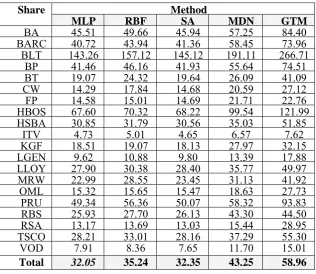
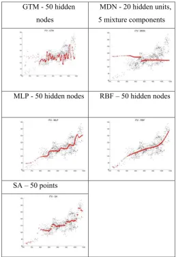
Table 1 represents the quantitative results for each method used, expressed as the mean error between actual and predicted stock prices over the considered period of time. Figure 1 illustrates the graphical results for the actual and the model output prices of one of the stocks - ITV obtained with the SA, MLP, RBF, MDN and GTM methods. These graphical results show the variation of the index value reflected on the prices of the this stock.
[image:6.595.132.452.413.684.2]The graphical and quantitative results corresponding to the SA, MLP and RBF models are comparable. The results obtained with the MDN method did not produce better representation of the data which again can be explained with the large dimensionality of the problem. In the case of the GTM method, although the quantitative results are worse than those obtained with the other methods, the graphical results show that the general trend of the actual prices is captured, demonstrating therefore the potential of the GTM method for modeling the distribution of the stock prices in terms of one latent variable.
Table 1. Mean error between actual and predicted prices of the 20 listed shares with different
methods
Method Share
MLP RBF SA MDN GTM
BA 45.51 49.66 45.94 57.25 84.40
BARC 40.72 43.94 41.36 58.45 73.96
BLT 143.26 157.12 145.12 191.11 266.71
BP 41.46 46.16 41.93 55.64 74.51
BT 19.07 24.32 19.64 26.09 41.09
CW 14.29 17.84 14.68 20.59 27.12
FP 14.58 15.01 14.69 21.71 22.76
HBOS 67.60 70.32 68.22 99.54 121.99
HSBA 30.85 31.79 30.56 35.03 51.85
ITV 4.73 5.01 4.65 6.57 7.62
KGF 18.51 19.07 18.13 27.97 32.15
LGEN 9.62 10.88 9.80 13.39 17.88
LLOY 27.90 30.38 28.40 35.77 49.97
MRW 22.99 28.55 23.45 31.13 41.92
OML 15.32 15.65 15.47 18.63 27.73
PRU 49.34 56.36 50.07 58.32 93.83
RBS 25.93 27.70 26.13 43.30 44.50
RSA 13.17 13.69 13.03 15.44 28.95
TSCO 28.21 33.01 28.16 37.29 55.30
VOD 7.91 8.36 7.65 11.70 15.01
The mean error = ( i=1,nabs(yi – ai))/n, where yi is the predicted and ai is the actual price of the shares, n is the total number days over which the share prices are predicted.
Fig. 1. Sample graphical result for the variation of the index value reflected on the ITV stock
price; the solid lines and the scattered dots indicate the predicted and actual stock prices respectively corresponding to the index values
GTM - 50 hidden nodes
MDN - 20 hidden units, 5 mixture components
MLP - 50 hidden nodes RBF – 50 hidden nodes
4 Conclusions
In this paper we investigate the use of a number of different techniques in the task of finding the mapping between a specific source of variation within a multivariate data distribution and the multivariate data distribution itself. The source of variation represents a quantity of interest related to a given problem domain. More specifically, we aim to define a mapping function relating the general index value among a set of shares to the prices of individual shares. We look for such mapping which gives a typical representation of the data distribution that exhibits the variation of the specific quantity. In this mapping, the target space has a higher dimension than the input space and for one input value the target output value is not unique. This leads to finding one-to-many multi-valued mapping. More specifically, we investigate several well-known methods used for solving such problems including MLP, RBF, MDN and GTM.
The results of our experiments demonstrate the potential of using neural networks trained with the MLP and RBF methods for isolating sources of variation and generating typical representations of the corresponding data distributions in the considered case study. With the neural network approach we do not make any assumptions about the mapping function; the neural networks are learning the complex mapping between the desired attributes and the parameters related the specific applications. The quantitative results obtained with the MLP and RBF are similar. The best result is achieved with the MLP method. The graphical results obtained with these methods are also similar. The MLP and RBF methods give the conditional averages of the target data conditioned on the input vectors and as expected they do not give a complete description of the target data reported in [4, 6]. For this problem we are addressing it is sufficient to define a mapping that generates typical samples of the data distribution (and not its entire variance) given specific values of the desired source of variation. This makes our results with the MLP and RBF (which are relatively simple methods, compared to MDN and GTM) not only acceptable but quite good for the type of inversion problems we are addressing, compared to the MLP results for the acoustic-to-articulatory inversion mapping reported in [14], [6]. For this one-to-many problem considered and also the problem of reconstructing the same spectrum from different spectral line parameters [4], the entire variance of the distribution is required. It has to be noted also that for the one-to-many problems considered in our paper the training algorithm for the MLP does not have to be modified as suggested by Brouwer [15], resulting in increased complexity. To the best of our knowledge RBFs have not previously been specifically used for one-to-many problems.
quantity of interest in the stock prices case study, they do not show complete representation of the target data space.
The GTM [5] is used to map points in the latent variable interval to points in the target data space and our results with this method actually show this mapping of one latent variable to the corresponding data spaces. It has to be noted though, that in order to isolate a specific source of variation, we need to find all latent variables which leads to a problem that is not computationally feasible [9]. In the stock price case study the isolated latent variable might be a different source of variation and not necessarily the desired index value.
The framework presented in the paper can be potentially useful in various applications involving multivariate distributions. With regards to the stock prices application, it is well established that trends of the general index can be easily predicted, unlike price fluctuations at share level. Therefore the ability to infer individual stock prices based on the general index value can be an invaluable tool for efficient portfolio management and prediction of the behaviour of individual shares.
References
1. Rumelhart, D.E., Hinton D.E., & Williams, R. J.: Learning representations by back-propagation errors. Nature, 323, pp. 533--536 (1986)
2. Powell, M.J.D.: Radial basis functions for multivariable interpolation: A review. IMA Conference on Algorithms for the approximation of Functions and Data (pp. 143-167). RMCS, Shrivenham, England (1985)
3. Bishop, C. M.: Neural Networks for Pattern Recognition. Oxford University Press, New York, Oxford (1995)
4. Bishop, C. M.: Mixture Density Networks. Technical Report NCRG/94/004, Neural Computing Research Group, Aston University,
research.microsoft.com/~cmbishop/downloads/Bishop-NCRG-94-004.ps (1994)
5. Bishop, C.M., Svensén, M., & Williams, C. K. I.: GTM: The Generative Topographic Mapping. Neural Computation, 10(1), pp. 215--234 (1998)
6. Richmond, K.: Mixture Density Networks, Human articulatory data and acoustic-to-articulatory inversion of continuous speech. URL
www.cstr.ed.ac.uk/downloads/publications/2001/Richmond_2001_a.ps (2001)
7. Bartholomew, D. J.: Latent Variable Models and Factor Analysis. Charles Griffin & Company Ltd, London (1987)
8. Dempster, A., Laird, N., & Rubin. D.: Maximum likelihood from incomplete data via the EM algorithm. Journal of the Royal Statistical Society. Series B, 39(1), pp. 1--38 (1977) 9. Carreira-Perpinan, M. A.: One-to-many mappings, continuity constraints and latent
variable models. In: Proc. IEE Colloquium on Applied Statistical Pattern Recognition, pp. 14/1--14/6, Birmingham (1999)
10. MacKay, D. J. C., & Gibbs, M. N.: Density networks. In: Proceedings of Society for General Microbiology. Edinburgh (1997)
11. Zeng, X. & Yeung D. S.: A Quantified Sensitivity Measure for Multilayer Perceptron to Input Perturbation. Neural Computation, 15, pp. 183--212 (2003)
12. FTSE Guide to UK Calculation Methods
http://www.ftse.com/Indices/UK_Indices/Downloads/uk_calculation.pdf#
14. Carreira-Perpiñán, M. Á.: Continuous latent variable models for dimensionality reduction and sequential data reconstruction. PhD thesis, Dept. of Computer Science, University of Sheffield, UK, faculty.ucmerced.edu/mcarreira-perpinan/papers/phd-thesis.html (2001) 15. Brouwer, R. K.: Feed-forward neural network for one-to-many mappings using fuzzy sets.