Finite time event triggered control and fault detection for singular Markovian jump mixed delay systems under asynchronous switching

R E S E A R C H

Open Access

Finite-time event-triggered control and

fault detection for singular Markovian jump

mixed delay systems under asynchronous

switching

Mengzhuo Luo

_{, Shouming Zhong}

_{and Jun Cheng}

*_{Correspondence:}

[email protected]

1_{College of Science, Guilin}

University of Technology, Guilin, P.R. China

Full list of author information is available at the end of the article

Abstract

This paper considers the problem of the simultaneous finite-time event-triggered control and fault detection for a class of continuous-time singular Markovian jump mixed delay systems (SMJDSs) under asynchronous switching. In order to develop the control and detection objectives, the mode-dependent fault detection filters and dynamic feedback event-triggered-based controllers are designed and the switching signal between the detector/controller unit and subsystems is assumed to be asynchronous. Based on average dwell time (ADT) techniques, some new sufficient conditions for the existence of fault detection/controller unit are presented in the framework of linear matrix inequalities (LMIs) to ensure the control system has singular stochastic finite-time stability (SSFTS). Finally, a numerical example is provided to illustrate the effectiveness of the proposed method.

Keywords: Detector/controller unit; Event-triggered control and fault detection; Singular stochastic finite-time stability; Asynchronous switching; Average dwell time

1 Introduction

In the past decade, the fault detection problem has been widely investigated due to the rising demand for higher safety and reliability standards in modern society. In generally, faults are unavoidable under practical conditions, such as hotspot faults, sensor faults and short circuits faults [1–3]. Up to now, various kinds of fault detection techniques have been developed, for example, model-based approaches, knowledge-based schemes and signal-based methods etc. Particularly, the problem ofH∞ optimization-based fault de-tection has been an active research area [4–7]. However, in many practical cases, the fault detection systems have feedback control, that is, the fault detection system is usually of closed-loop type, and if the fault detection systems are designed separately from the con-trol algorithms, faults may be hidden by concon-trol actions and the early detection of faults is clearly more difficult, especially low frequency faults [8–15]. Therefore, the problem of merging the control and fault detection units into a single detector/controller unit, i.e. si-multaneous control and fault detection issue has become a very important research topic in information security field; recently. [8] dealt with the problem of simultaneous finite-time control and fault detection for linear switched systems with state delay and parameter

uncertainties; [9] was concerned with the simultaneous robust control and fault detection problem for continuous-time switched systems subject to dwell time constraint; [10] in-vestigated the problem of simultaneous fault detection and control for switched linear systems under a mixedH∞/H–framework and [11] presented the problem of

simultane-ous fault detection and control design for switched systems with two quantized signals; in [12], the authors first attempted to deals with the simultaneous robust fault detection and control problem for a class of nonlinear stochastic switching systems under asynchronous switching; this paper further improved the results in the literature [9].

In practical situations, the periodical sampling is often used to control physical plants since it can simplify the design and analysis [16]. However, the communication burden is neglected in the framework of the periodic sampling; especially when the difference between consecutive sample-data is not distinct, it is obviously a waste of limited com-munication resources transmitting the sampled data to the controller [17]. Recently, in order to overcome this difficulty, event-triggered scheme is introduced and has been re-ceived particular attention, which is more convenient and effective than the traditional time-triggered technique, meantime, compared with the time-triggered mechanism, the event-triggered scheme can promise energy efficiency and reduce the burden of the com-munication [18–21].

In most existing literature, finite-time stability has received increasing attention and the concept of finite-time stability was proposed in practical processes, such as avoiding saturation or the excitation of nonlinear dynamics during the transient [22, 23]. Differ-ent from the classical Lyapunov stability concept, finite-time stability is defined as the behavior of the dynamical systems that can be tracked over a fixed finite-time interval, that is, the system state does not exceed a certain bound during a fixed finite-time inter-val. The introduction of such a stability concept is very necessary and important in many practical problems. So, the problem of finite-time stability it is not only the need of theo-retical learning, but also the need of practical application. Now, many interesting results have been obtained for this type of stability. For example, [24] investigated the problem of robust finite-time boundedness ofH∞filtering for switch systems with time-varying delay; [25] addressed a finite-time stabilization problem for a class of continuous-time Markovian jump delay systems with switching control approach; [26] studied observer-based state feedback finite-time control for nonlinear jump systems with time-delay and [27] dealt with the finite-time synchronization problem for a class of uncertain coupled switched neural networks under asynchronous switching.

the major issues of stability and control analysis for time-delay singular systems has been studied extensively in actual problems [30, 31].

The main challenge is now simultaneous finite-time control and fault detection in the presence of some complicated factors, such as jump model uncertainty, mixed delay and disturbances for a class of singular Markovian jump delay systems under asynchronous switching. To the best of our knowledge, this problem has not been investigated yet. Therefore, motivated by the aforementioned observations, in this paper, we will deal with the problem of simultaneous finite-time event-triggered control and fault detection for a class of singular Markovian systems with asynchronous switching signal, which based on some novel integral inequalities and average dwell time method. The purpose of this paper is to design mode-dependent detector/controller unit such that the augmented sys-tem is not only singular stochastic finite-time stability but also satisfiesH∞performance indices. A novel stochastic Lyapunov function and a set of strict LMIs will be utilized to derive sufficient conditions guaranteeing the desired detector/controller unit can be con-structed. The main contributions of this paper can be summarized as follows: (1) In this paper, a class of much more general singular systems including both stochastic switch, de-terministic switch and mixed time-varying delay are considered simultaneously. (2) Based on the event-triggered scheme, the simultaneous finite-time control and fault detection problem under asynchronous switching for a class of singular Markovian jump system is considered for the first time. (3) Compared with the method in [8], some novel suf-ficient conditions for singular stochastic finite-time stability of Markovian jump systems are obtained in this paper by virtue of new integral inequalities and asynchronous analysis method. (4) A mode-dependent controller/detector, which subject to the ADT constraint is designed, the elements of the transition rate matrix is modeled as a function of the high-level switching signalϑt=p,ϑ˜t=q; furthermore, owing to the bounded uncertainty description, the uncertainty entry in the transition rate matrix is represented by its upper and lower bounds.

Notations The notations are quite standard. Throughout this letterRn_andRn×m de-note, respectively, the n-dimensioned Euclidean space and the set of alln×mreal matri-ces. The notationX≥Y (respectively,X>Y) means thatXandYare symmetric matri-ces, and thatX–Y is positive semi-definitive (respectively, positive definite).L2[0, +∞) is square integrable function vector over [0, +∞). · is the Euclidean norm inRn_.Iis the identity matrix with appropriate dimensions. X+XT _{is denotedHe(X) for} simplic-ity. IfAis a matrix,λmax(A) (respectively,λmin(A)) means the largest (respectively,

small-est) eigenvalue ofA. Moreover, let (,F, (Ft)t≥0,P) be a complete probability space with a filteration. (Ft)t≥0 satisfies the usual conditions (i.e., the filtration contains allP-null sets and is right continuous).E{·}stands for the mathematical expectation operator with respect to the given probability measure. Denote by L2_F0([–dτ, 0] :Rn) the family of all F0measurableC([–dτ, 0] :Rn)-valued random variablesϕ={ϕ(s) : –dτ≤s≤0}such that sup_–d

τ≤s≤0Eϕ(s)

2_{<∞. The asterisk∗in a matrix is used to denote a term that is induced}

2 Problem formulation and preliminaries

Consider a class of SMJDSs described by the following model:

⎧ ⎪ ⎪ ⎪ ⎪ ⎪ ⎪ ⎪ ⎪ ⎨ ⎪ ⎪ ⎪ ⎪ ⎪ ⎪ ⎪ ⎪ ⎩

E(ϑt)x˙(t) =A(υt,ϑt)x(t) +Ad(υt,ϑt)x(t–d(t)) +Aτ(υt,ϑt) t

t–τ(t)x(s)ds

+B(υt,ϑt)u(t) +Bh(υt,ϑt)h(t) +Bf(υt,ϑt)f(t),

y(t) =C1(ϑt)x(t) +D(ϑt)x(t–d(t)) +Dτ(ϑt) t

t–τ(t)x(s)ds+Dh(ϑt)h(t)

+Df(ϑt)f(t),

x(t) =φ(t), t∈[–dτ, 0],

(1)

where x(t)∈Rn _{is the system state vector,y(t)∈R}m _{is the measured output,h(t)∈R}l is disturbance input,u(t)∈Rg _{is the control input andf(t)∈R}v_{is the fault vector. The} matrixE(ϑt)∈Rn×nmay be singular, and it is assumed thatrank(E(ϑt)) =r≤n.φ(t) is a vector-valued initial continuous function defined on the interval [–dτ, 0].ϑtis a piecewise constant switching signal taking values in 1={1, 2, . . . ,ι},ι∈N. Supposet0<t1<· · · is

the switching sequence, then the system switches at instantst0<t1<· · ·, andϑ(t) =ϑ(tl) for∀t∈[tl,tl+1), andl= 0, 1, . . . .

Assumption 2.1 The input matrices B(υt,ϑt)are full column rank and therefore,there

exists nonsingular matricesT¯(υt,ϑt)such thatT¯(υt,ϑt)B(υt,ϑt) = I

0

.

Assumption 2.2 In this paper,the time-varying delays d(t),τ(t)are continuous satisfying

0≤d1≤d(t)≤d2,d˙(t)≤d< 1and0≤τ1≤τ(t)≤τ2,where d1,τ1and d2,τ2are constants involving the lower and the upper bounds of the delays,dτ =max{d2,τ2},d¯=d2–d1,τ¯=

τ2–τ1.

In this paper, the aim is to design a detector (filter)/controller (state feedback) unit, which is described by

⎧ ⎪ ⎪ ⎨ ⎪ ⎪ ⎩

E(ϑ˜t)x˙f(t) =Aˆ(υt,ϑ˜t)xf(t) +Bˆ(υt,ϑ˜t)y(t),

r(t) =Cˆr(υt,ϑ˜t)xf(t) +Dˆr(υt,ϑ˜t)y(t),

u(t) =Kˆ(υt,ϑ˜t)xf(˜tσ), t∈[˜tσ,t˜σ+1),∀σ∈N,

(2)

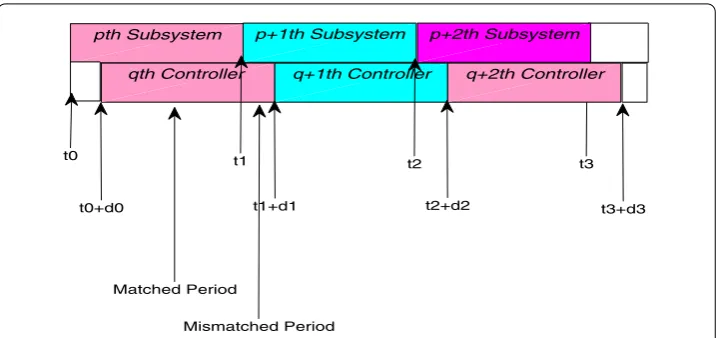
wherexf(t)∈Rnis the state of the detector/controller unit,r(t)∈Rl1is the residual signal, the matricesAˆ(υt,ϑ˜t),Bˆ(υt,ϑ˜t),Cˆr(υt,ϑ˜t),Dˆr(υt,ϑ˜t) andKˆ(υt,ϑ˜t) are detector/controller gains, which will be determined. Moreover,ϑ˜tis the switching signal of detector/controller unit and can be regarded as a delayed signal ofϑt. Under the switching signalϑtandϑ˜t, one can get the following switching sequences and Fig. 1 shows the phenomenon of asyn-chronous switching:

⎧ ⎨ ⎩

ϑt:{(t0,ϑ(t0)), (t1,ϑ(t1)), . . . , (tk,ϑ(tk)), . . .},

˜

ϑt:{(t0,ϑ(t0)), (t1+d1,ϑ(t1)), . . . , (tk+dk,ϑ(tk)), . . .},

(3)

Figure 1Asynchronous switching between subsystem and controller unit

instant of detector/controller unit to that of the system (1), and it is assumed that d˜= max{dk|k= 0, 1, . . .}cannot exceed the next switching instant of the system.

{υt,t≥0}is a continuous-time discrete state Markov process with right continuous tra-jectory values in a finite setK={1, 2, . . . ,k˜},k˜∈Nwith the TPs

Pr(υt+ =j|υt=i,ϑt=p,ϑ˜t=q) = ⎧ ⎨ ⎩

π_ij(pq) +o( ), i=j,

1 +π_ii(pq) +o( ), i=j, (4)

where > 0,lim _→0+o( )/ = 0 andπ(pq)

ij is the transition rate from modeiat timetto modejat timet+ that satisfiesπ_ij(pq)> 0,π_ii(pq)= – k_j˜_{=1,j =i}π_ij(pq)(∀i,j∈K,∀p,q∈ 1).

Remark2.1 Based on the definition of the transition rate matrix(pq), we know that every elementπ_ij(pq)of the matrix(pq)is a function of the switch modeϑt=p,ϑ˜t=q, it means that this matrix can be defined as

(pq)= ⎡ ⎢ ⎢ ⎣

π₁₁(pq) · · · π(pq) 1˜k ..

. . .. ...

π(_˜pq)

k1 · · · π (pq) ˜

kk˜ ⎤ ⎥ ⎥

⎦. (5)

Note that matrix(pq)is the varying and subject to the ADT constraint. Such time-varying transition ratesπ_ij(pq) are unknown but they belong to the admissible bounded compact set

π_ij(pq)=π¯_ij(pq)+ π¯_ij(pq) (6)

and the uncertain π¯_ij(pq)belongs to the range of [–δ_ij(pq),δ_ij(pq)], whereδ_ij(pq)> 0, for alli,j∈

K,p,q∈ 1. The entry ofπ¯ij(pq)andδ

(pq)

ij satisfyπ¯

(pq)

ii = –

˜

k j=1

j =i

¯

π_ij(pq),δ(_iipq)= kj˜=1

j =i

δ_ij(pq).

Now, we will introduce the following event-trigger instant sequence:

χ=[˜t0,˜t1), [t1˜,t2˜), . . . , [˜tσ,˜tσ+1), . . .|σ∈N

Without loss of generality, we assume that the first event happens at time instantt0˜. With the system state estimates xf(˜tσ) sampled at time instant˜tσ, the next sampling instant

˜

tσ+1can be determined by the event-trigger. In this paper, the state feedback controller is

event-triggered, which can be given by

u(t) =Kˆ(υt,ϑ˜t)xf(˜tσ), t∈[˜tσ,˜tσ+1),∀σ∈N. (8)

Note that in the event-triggered scenario, at sampling time instant˜tσ, the controller (8) will receive the sampled data and hold unchanged until next event is generated at time instant˜tσ+1, that is, there is no new control input updates during two consecutive time

instants in sequenceχ. Hence, a zero-order holder (ZOH) is equipped in the system in order to keep the control signal continuous.

Now, we introduce the event detector which is used to determined whether the newly sampled data should be sent out to the controller by using the following threshold condi-tion:

eT(t)1ie(t) –ρixTf (t)2ixf(t)≤0, (9)

wheree(t) =xf(t˜σ) –xf(t),1i> 0 and2i> 0 for eachi∈K, are an event-triggered weight-ing matrix to be determined for a proper error toleranceρi∈[0, 1). Based on the above inequality, we know that if the sampling data exceeds the threshold condition (9), the (σ+ 1)th event will be triggered.

Remark 2.2 Based on (9), we know that the next event will not be generated before

eT_(t)1

ie(t) –ρixT_f(t)2ixf(t) = 0 and at the event-trigger instant˜tδ, ife(t) = 0, one sees that a positive lower bound exists on the inter-event, that is, ˜tδ+1–t˜δ > 0, which elimi-nates the Zeno behavior of the sampling. Furthermore, by the similar method, which was discussed in [18], a positive lower bound will be obtained. Therefore, based on the above description, the Zeno behavior of the sampling can be excluded because there is no accu-mulation point in the sampling if

˜ tδ+1=inf

t>˜tδ|eT(t)1ie(t) –ρixTf(t)2ixf(t)≥0

∀δ∈N

holds.

Then, by combining the detector/controller unit (2) and the system (1), we can obtain the following augmented system:

⎧ ⎪ ⎪ ⎪ ⎪ ⎪ ⎨ ⎪ ⎪ ⎪ ⎪ ⎪ ⎩

˜

Epqx˙˜(t) =A˜ipqx˜(t) +A˜dipqx˜(t–d(t))

+A˜τipq t

t–τ(t)x˜(s)ds+A˜eipqe(t) +B˜zipqz(t), ˆ

r(t) =C¯ripqx˜(t) +DˆriqDpkx˜(t–d(t))

+DˆriqDτpk t

t–τ(t)x˜(s)ds+D¯ripqz(t) –Cwxw(t).

(10)

CaseI:switching signalsϑtandϑ˜tare a mismatch,then

˜ Epq=

Ep 0

0 Eq

, A˜ipq=

Aip BpKˆiq

ˆ

BiqC1p Aˆiq

, A˜dipq=

Adip 0

ˆ BiqDp 0

˜

Remark2.3 In this paper, the simultaneous finite-time control and fault detection prob-lem will be described as designing a detector/controller unit in form of (2) such that the augmented system (10) is SSFTS and the followingH∞ property should be guaranteed

when there exists a disturbance and fault under zero initial conditions:

E T

investi-gated yet, and the results show great room to improve by introducing some novel integral inequalities. So, this is the main motivation for us to further develop the simultaneous finite-time control and fault detection problem.

Now, the following definitions are given, which are indispensable for later develop-ment.

Definition 2.1([32]) For any switching signal and anyk0<ks<k, letNδ(ks,k) denote the number of switching signals over the time interval [ks,k). For givenN0> 0,τa> 0, then

Nδ(ks,k)≤N0+ k–ks

τa

, (13)

whereτais called average dwell time andN0denotes the chatter bound.

Definition 2.2([33]) systemE˜pqx˙˜(t) =A˜ipqx˜(t) (or pair (E˜pq,A˜ipq)) is said to be:

1. regular ifdet(zE˜pq–A˜ipq)is not identically zero for anyi∈K,p,q∈ 1;

2. impulse-free if it is regular and degree(det(zE˜pq–A˜ipq)) =rank(E˜pq)for anyi∈K,

p,q∈ 1.

Definition 2.3 ([34]) The augmented system (10) is said to be SSFTS with respect to (c1,c2,G,T). With 0 <c1<c2,G > 0, if the stochastic system is regular and impulse-free in timet∈[t0,T] and satisfies

sup t0–dτ≤t≤0

Ex˜T(t)Gx˜(t),xT_w(t)Gxw(t),x˙˜T(t)Gx˙˜(t)

≤c1

⇒ Ex˜T(t)Gx˜(t)<c2, t∈[t0,T]. (14)

Before proceeding, we will introduce the following lemmas which will play an important role in the derivation of our main results.

Lemma 2.1([35]) For a differentiable function x: [α,β]→Rn,a positive definite matrix R∈Rn×n_{,a vectorξ∈R}k_{,and any matrices N}

i∈Rn×n(i= 1, 2),the following inequality

hold:

– β

α

˙

xT(s)Rx˙(s)ds

≤ξT

(α–β)

N1R–1N₁T+1 3N2R

–1_NT

2

+He(N1E1+N2E2)

ξ, (15)

where

E1ξ=ϒ1(α,β) =x(β) –x(α),

E2ξ=ϒ2(α,β) =x(β) +x(α) –

2

β–α

β

α

Lemma 2.2 For any appropriately dimensioned matrices Z=ZT_{> 0,Z∈R}n×n_,M∈Rm×n

and positive scalars d1,andα,the following inequality holds:

– t

t–d1

eα2(t–s)_x˙˜T_(s)E˜T_ZE˜_x˙˜_(s)ds

≤ξT(t)εMZ–1MT_{ξ(t) + 2ξ}T_(t)ME˜_{x˜(t) –E}˜_x˜(t–d

1)

,

(16)

whereε= 1

α2(1 –e –α2d1_).

Proof Firstly, we can find that the following inequality is true

t

t–d1

ξ(t)

˜ Ex˙˜(s)

T

e–α(t2–s)_M eα(t2–s)_Z

Z–1

e–α(t₂–s)_MT _eα(t₂–s)_Z ξ(t)

˜ Ex˙˜(s)

ds≥0, (17)

which implies the inequality (16) is satisfied.

Remark2.5 Lemma 2.1 and Lemma 2.2 represent some novel results to handle the integral term of quadratic quantities in the estimation of LKF derivative. Lemma 2.1 includes more information of state and time-varying delay into the augmented vectorsξ(t); Lemma 2.2 contains the exponential information, and it does not use the approximation –eα(t–s)_{< –1,} t–d2≤s≤t–d1, which presents less precision. So, Lemma 2.1 and Lemma 2.2 are helpful

to reduce the imprecision of our results.

Lemma 2.3([36]) For any constant matrix M> 0,any scalars a and b with a<b,and a

vector function x(t) : [a,b]→Rnsuch that the integrals concerned are well defined,then the following inequality holds:

b

a

x(s)ds

T

M

b

a

x(s)ds

≤(b–a) b

a

xT(s)Mx(s)ds. (18)

3 Design of the detector/controller unit

In this section, LMI conditions are presented such that the SSFTS and performance property (12) are satisfied simultaneously for augmented system (10) with average dwell time constraint and then we will endeavour to develop the design problems for detec-tor/controller unit with the form of (2).

Theorem 3.1 For any i,j∈K,p,q∈ 1,α1> 0,α2> 0,γ0> 0,and given matricesAˆiq,

ˆ

Biq,Cˆriq,Dˆriq,Kˆiq,R˜pq,then the augmented system(10)with z(t) = 0is SSFTS with respect given(c1,c2,G,T)and the performance index(12)is satisfied,if there exist positive definite matrices Pipq,Pwpq,Qlpq,l= 1, 2, 3,R1¯ pq,R2¯ pq,W1pq,W1¯ pq,W21pq,W22pqsymmetric matrices

W21pq H1

H1 W22pq

> 0,

W21pq H2

H2 W22pq

> 0,

⎡ ⎢ ⎢ ⎢ ⎢ ⎣

W21pq H1

H1 W22pq

G

GT

W21pq H2

H2 W22pq

⎤ ⎥ ⎥ ⎥ ⎥ ⎦> 0,

(23)

η1c2e–α1Tm(t0,T)–α2Tmism(t0,T)_{>η2c1, (24)}

and the average dwell time satisfying

τa>τa∗

=max

(ln(μ1μ2) +|α1–α2|dτ)T lnc2

c1 +ln

η1

η2 –α1Tm(t0,T) –α2Tmism(t0,T)

,

ln(μ1μ2) +|α1–α2|dτ+α2d˜ α1

, (25)

where

(₁₁pq)=He(MipqA˜ipq) –α2E˜pqTPipqE˜pq+

3

v=1

Qvpq+τ12R1¯ pq

+τ¯2R2¯ pq+He(T51E˜pq) +ρikT2ik+d¯2E˜pqTW21pqE˜pq

+

˜

k

j=1

j =i

¯

π_ij(pq)E˜T_pq(Pjpq–Pipq)E˜pq+

˜

k

j=1

j =i 1 4

δ_ij(pq)2εij,

(₁₂pq)=MipqA˜dipq, 13(pq)= –T51E˜pq+E˜pqTT53T, (pq) 15 =

0 MipqA˜τipq 0

,

(₁₇pq)=0 0 MipqA˜eipq MipqB˜zipq

, (₁₈pq)=C¯T

ripq A˜Tipq 0n×2n T51

,

(₁₉pq)=E˜T

pq(P1pq–Pipq)E˜pq · · · ˜EpqT(P(i–1)pq–Pipq)E˜pq E˜Tpq(P(i+1)pq–Pipq)E˜pq

· · · ˜ET

pq(P˜kpq–Pipq)E˜pq

,

(₂₂pq)= –(1 –d)e–α2d2_Q1

pq+He

T12E˜pq+T22E˜pq–T32E˜pq+T42E˜pq–E˜TpqG2E˜pq

+E˜T_pq(d¯H1–d¯H2)E˜pq+ 2E˜pqTW22pqE˜pq,

(₂₃pq)=T32E˜pq–E˜TpqT33T +T42E˜pq+E˜pqTT43T +E˜TpqG2E˜pq–E˜pqTW22pqE˜pq,

(₂₄pq)= –T12E˜pq+E˜TpqT14T+T22E˜pq+E˜TpqT24T +E˜pqTGT2E˜pq–E˜pqTW22pqE˜pq,

₂₇(pq)=–T22E˜pq+E˜pqTT210T –d¯E˜TpqH1E˜pq –T42E˜pq+E˜TpqT411T +d¯E˜TpqH2E˜pq 0 0

,

(₂₈pq)=

(DˆriqDpk)T A˜T_dipq dT12¯ dT22¯ 0

,

(₃₃pq)= –eα2d1_Q2

pq+He(T33E˜pq+T43E˜pq–T53E˜pq) +E˜Tpq(d¯H2+W22pq)E˜pq(34pq)

= –E˜T_pqGT₂E˜pq,

(₃₇pq)=0 –T43E˜pq+E˜pqTT411T –d¯E˜TpqH2E˜pq 0 0

, (₃₈pq)=0n×4n T53

(₄₄pq)= –eα2d2_Q3

and positive scalarα1in the LMIs(19)and(20),we can obtain the LMIs(21)and(22), respectively.

Proof In order to develop our results, we will divide the time interval into two parts, one is [tk,tk+dk) (k= 0, 1, . . .), the other is [tk+dk,tk+1) (k= 0, 1, . . .), which correspond to the

asynchronous and synchronous time interval between the switched subsystems and their controller unit, respectively. Next we will discuss our problems in two cases.

Firstly, we will show that the system (10) is regular and impulse-free. From (19), it is seen

whereU˜pqis any real nonsingular matrix for anyp,q∈ 1. Now, we will pre-multiplying

and post-multiplying(₁₁pq)< 0 by N˜T andN˜, we can haveHe(Spq2U˜pqA˜(22)ipq) < 0, which impliesA˜(22)_ipq is nonsingular matrix. Then, fori∈K,p,q∈ 1, pair (E˜pqA˜ipq) is regular and impulse-free. Based on Definition 2.2, we can see that augmented system (10) is regular and impulse-free for any time-varyingd(t) satisfying Assumption 2.2.

Now, we will show augmented system (10) is SSFTS. Firstly, choose a stochastic Lya-punov function candidate for the system (10) for anyi∈K,p,q∈ 1:

– (1 –d)e–α2d2_x˜T_t–d(t)Q1

Now, from Lemma 2.1 and Lemma 2.2, we have

T₃T=0 TT

×

Based on the reciprocally convex approach, for any matrixG, we can obtain the follow-ing inequality:

Next, in order to deduce our results, we suppose that

ϒ(t) =γ₀2zT_{(t)z(t) –ˆr}T_{(t)rˆ(t). (36)}

In view of event condition (9),eT_(t)

1ie(t) –ρixT_f(t)2ixf(t)≤0 holds for allt≥0 and combining the above discussion by the Schur complement lemma, it can be deduced that

LVpq(t) –α2Vpq(t) –ϒ(t) < 0, (37)

if inequalities (19) and (20) are satisfied.

CaseII:In match period.

Fort∈[tk+dk,tk+1) (k= 0, 1, . . .), which is the synchronous time interval between the

switched subsystems and their controller unit. Next, similar to Case I, we will further ana-lyze our results under the match period. Let choose the following multiple Lyapunov-like functional for the augmented system (10) as

V_p(1)(t) =x˜T(t)E˜T_pPipE˜px˜(t), (38)

V_p(2)(t) = t

t–d(t)

eα1(t–s)_x˜T_(s)Q1

px˜(s)ds+ t

t–d1

eα1(t–s)_x˜T_(s)Q2

px˜(s)ds

+ t

t–d2

eα1(t–s)_x˜T_(s)Q3

px˜(s)ds, (39)

V_p(3)(t) =τ1

0

–τ1

t

t+θ

eα1(t–s)_x˜T_(s)R1¯

px˜(s)ds dθ

+τ¯

–τ1

–τ2

t

t+θ

eα1(t–s)_x˜T_(s)R2¯

px˜(s)ds dθ, (40)

V_p(4)(t) = 0

–d1

t

t+θ

eα1(t–s)_x˙˜T_(s)E˜T

pW1¯ pE˜px˙˜(s)ds dθ

+ –d1

–d2

t

t+θ

eα1(t–s)_x˙˜T_(s)E˜T

pW1pE˜px˙˜(s)ds dθ, (41)

V_p(5)(t) =d¯

–d1

–d2

t

t+θ

eα1(t–s)

˜ Epx˜(s)

˜ Epx˙˜(s)

T

W21p 0

0 W22p

˜ Epx˜(s)

˜ Epx˙˜(s)

ds dθ, (42)

V_pq(6)=

xw(t)

˙ xw(t)

T

Pwp 0

0 Swp

I 0

0 0

xw(t)

˙ xw(t)

. (43)

Similar to the proof of Case I, if (21) and (22) hold, then

LVp(t) –α1Vp(t) –ϒ(t) < 0. (44)

Then from (37) and (44), we can have

EV(t)≤ ⎧ ⎪ ⎪ ⎪ ⎪ ⎪ ⎨ ⎪ ⎪ ⎪ ⎪ ⎪ ⎩

eα2(t–tk)E{_Vpq(tk)}

+E{_tt ke

α2(t–s)_ϒ(s)ds}_{, t}∈_[tk,t

k+dk) (k= 0, 1, . . .),

eα1(t–(tk+dk))E{_Vp(t k+dk)}

+E{_tt k+dke

α1(t–s)_ϒ(s)ds}_{, t}∈_[t

k+dk,tk+1) (k= 0, 1, . . .).

Step1. Firstly, we will show that the augmented system (10) is SSFTS under the condi-tions of Theorem 3.1 ifz(t) = 0.

Based on the truth of (37) and (44), we know that ifz(t) = 0, (45) is equivalent to

EV(t)≤ ⎧ ⎨ ⎩

eα2(t–tk)E{_Vpq(tk)}_{, t}∈_[tk,t

k+dk) (k= 0, 1, . . .),

eα1(t–(tk+dk))E{_V

p(tk+dk)}, t∈[tk+dk,tk+1) (k= 0, 1, . . .).

(46)

Without loss of generality, one assumes thatα1≥α2and the other condition ofα1<α2

will be analyzed in the following.

From the definitions ofVpq(t) andVp(t), it shows that ifα1≥α2,

EVpq(t)≤μ1EVp(t) EVp(t)≤μ2edτ(α1–α2)E_{Vpq(t), (47)}

where

μ1=max

_max

p,q∈ 1,i∈˜k(λmax(E˜

T

pqPipqE˜pq))

min_p∈

1,i∈˜k(λmin(E˜TpPipE˜p))

,maxp,q∈ 1(λmax(Pwpq))

min_{p∈ 1}(λmin(Pwp)) ,

maxp,q∈ 1(λmax(Q1pq))

minp∈ 1(λmin(Q1p))

,maxp,q∈ 1(λmax(Q2pq))

minp∈ 1(λmin(Q2p))

,maxp,q∈ 1(λmax(Q3pq))

minp∈ 1(λmin(Q3p))

,

maxp,q∈ 1(λmax(R1¯ pq))

minp∈ 1(λmin(R1¯ p))

,maxp,q∈ 1(λmax(R2¯ pq))

minp∈ 1(λmin(R2¯ p))

,maxp,q∈ 1(λmax(E˜ T

pqW1pqE˜pq))

minp∈ 1(λmin(E˜TpW1pE˜p)) ,

maxp,q∈ 1(λmax(E˜

T

pqW1¯ pqE˜pq)) minp∈ 1(λmin(E˜TpW1¯ pE˜p))

,maxp,q∈ 1(λmax(E˜ T

pqW21pqE˜pq)) minp∈ 1(λmin(E˜pTW21pE˜p))

,

max_{p,q∈ 1}(λmax(E˜TpqW22pqE˜pq)) minp∈ 1(λmin(E˜TpW22pE˜p))

(48)

μ2=max

_max

p∈ 1,i∈˜k(λmax(E˜TpPipE˜p)) min_p,q∈

1,i∈˜k(λmin(E˜

T

pqPipqE˜pq))

, maxp∈ 1(λmax(Pwp)) minp,q∈ 1(λmin(Pwpq))

,

maxp∈ 1(λmax(Q1p))

min_{p,q∈ 1}(λmin(Q1pq))

, maxp∈ 1(λmax(Q2p))

min_{p,q∈ 1}(λmin(Q2pq))

, maxp∈ 1(λmax(Q3p))

min_{p,q∈ 1}(λmin(Q3pq)) ,

maxp∈ 1(λmax(R1¯ p))

minp,q∈ 1(λmin(R1¯ pq))

, maxp∈ 1(λmax(R2¯ p))

minp,q∈ 1(λmin(R2¯ pq))

, maxp∈ 1(λmax(E˜ T

pW1pE˜p)) min_{p,q∈ 1}(λmin(E˜TpqW1pqE˜pq))

,

maxp∈ 1(λmax(E˜

T

pW1¯ pE˜p)) minp,q∈ 1(λmin(E˜TpqW1¯ pqE˜pq))

, maxp∈ 1(λmax(E˜ T

pW21pE˜p)) minp,q∈ 1(λmin(E˜TpqW21pqE˜pq))

,

maxp∈ 1(λmax(E˜TpW22pE˜p)) minp,q∈ 1(λmin(E˜TpqW22pqE˜pq))

. (49)

Then, for anyt∈[tk,tk+dk) andα1≥α2, we can obtain

EV(t)≤eα2(t–tk)E_Vpq(tk)≤_μ1eα2(t–tk)E_V p

t–_k

≤μ1eα2(t–tk)_eα1(tk–(tk–1+dk–1))E_Vp(t

k–1+dk–1)

≤μ1eα2(t–tk)_eα1(tk–(tk–1+dk–1))_μ2edτ(α1–α2)E_Vpq(t

k–1+dk–1)–

≤μ1eα2(t–tk)_eα1(tk–(tk–1+dk–1))_μ2edτ(α1–α2)_eα2(tk–1+dk–1–tk–1)E_Vpq(t

k–1)

≤ · · · ≤μNϑ(t0,t)

1 μ

Nϑ˜(t_0,t)

2 e

Nϑ˜(t0,t)dτ(α1–α2)_eα2(t–tk+dk–1+dk–2+···+d0)

×eα1(tk–dk–1–dk–2–···–d0–t0)E_V(t0).

It is easy to obtain the following fact through simple calculations:

t–tk+dk–1+dk–2+· · ·+d0<dk+dk–1+dk–2+· · ·+d0=Tmism(t0,t), (50)

tk–dk–1–dk–2–· · ·–d0–t0

= (tk–tk–1–dk–1) + (tk–1–tk–2–dk–2) +· · ·+ (t1–t0–d0) =Tm(t0,t), (51)

whereTmism(t0,t) andTm(t0,t) denote the total mismatched time and matched time in-terval lengths on [t0,t].Nϑ(t0,t)andNϑ˜(t0,t)denote the number of synchronous and

asyn-chronous switching on the interval [t0,t), respectively. Furthermore, based on the

assump-tion ofdmax, we know that relational expressionNϑ˜(t0,t)<Nϑ(t0,t)is true.

In conclusion, it gives that

EV(t)≤μNϑ(t0,t)

1 μ

Nϑ(t0,t)

2 eNϑ(t0,t)dτ(

α1–α2)_eα2Tmism(t0,t)_eα1Tm(t0,t)E_V(t 0)

. (52)

Next, ifα1<α2, we can also obtain following inequalities very easily by the similar

anal-ysis in (47):

EVp(t)≤μ2E

Vpq(t), EVpq(t)≤μ1edτ(α2–α1)E_{Vp(t). (53)}

According to the same techniques as in the proof of (52), the following inequality is true

EV(t)≤μNϑ(t0,t)

1 μ

Nϑ(t_0,t)

2 e

Nϑ(t0,t)dτ(α2–α1)_eα2Tmism(t0,t)_eα1Tm(t0,t)E_{V(t0). (54)}

By combining the two cases withα1≥α2andα1<α2, eventually, we have the estimation

ofE{V(t)}as follows:

EV(t)≤μNϑ(t0,t)

1 μ

Nϑ(t0,t)

2 eNϑ(t0,t)dτ|

α1–α2|_eα2Tmism(t0,t)_eα1Tm(t0,t)E_V(t 0)

. (55)

According to the definition ofV(t), we know that

EV(t)≥η1E

˜

xT(t)Gx˜(t), (56)

where

η1=min

_min

p,q∈ 1,i∈˜k(λmin(E˜

T

pqPipqE˜pq))

λmax(G)

,minp∈ 1,i∈˜k(λmin(E˜

T pPipE˜p))

λmax(G)

and

whereα¯=max{α1,α2},

η2=

_max

p,q∈ 1,i∈˜k(λmax(E˜

T

pqPipqE˜pq))

λmin(G)

+e

¯

αd2_(max

p,q∈ 1(λmax(Q1pq)) +maxp,q∈ 1(λmax(Q3pq))) λmin(G)

+e

¯

αd1_(max

p,q∈ 1(λmax(Q2pq)))

λmin(G)

+e

¯

ατ1_τ2

1maxp,q∈ 1(λmax(R1¯ pq))

λmin(G)

+e

¯

ατ2_τ¯2_max

p,q∈ 1(λmax(R2¯ pq)) λmin(G)

+e

¯

αd2_d¯2_max

p,q∈ 1(λmax(E˜pqTW21pqE˜pq))

λmin(G)

+e

¯

αd2_d¯_max

p,q∈ 1(λmax(E˜TpqW1pqE˜pq))

λmin(G)

+maxp,q∈ 1(λmax(Pwpq)) λmin(G)

+e

¯

αd1_d

1maxp,q∈ 1(λmax(E˜

T

pqW¯1pqE˜pq))

λmin(G)

+e

¯

αd2_d¯2_max

p,q∈ 1(λmax(E˜

T

pqW22pqE˜pq))

λmin(G)

. (58)

Then for anyt∈[t0,T], we can conclude that

Ex˜T(t)Gx˜(t)≤(μ1μ2) T τa_e

T

τa|α1–α2|dτ_eα1Tm(t0,T)+α2Tmism(t0,T)_η2c1 η1

. (59)

Therefore, from (24), (25), we can haveE{˜xT_{(t)Gx˜(t)}<c}

2, then, according to

Defini-tion 2.3, system (10) is SSFTS under the asynchronous switching.

Step2. In this section, we will show thatH∞ property (12) should be guaranteed if the conditions of Theorem 3.1 are satisfied.

Firstly, according to the (45) and the similar proof ofStep1, we can conclude that

EV(t)≤μ1μ2e|α1–α2|dτ

Nϑ(t0,t)

eα1Tm(t0,t)+α2Tmism(t0,t)_EV(t 0)

×E t

t0

μ1μ2e|α1–α2|dτ

Nϑ(s,t)

eα1Tm(s,t)+α2Tmism(s,t)_ϒ(s)ds

. (60)

FromE{V(t)} ≥0, (60) implies that under zero initial conditions and fort0= 0

E t

0

eln(μ1μ2+e|α1–α2|dτ)Nϑ(s,t)

eα1Tm(s,t)+α2Tmism(s,t)_rˆT_(s)rˆ_(s)ds

≤γ₀2E

t

0

eln(μ1μ2+e|α1–α2|dτ)Nϑ(s,t)_eα1Tm(s,t)+α2Tmism(s,t)_zT_(s)z(s)ds

≤γ₀2E

t

0

eln(μ1μ2+e|α1–α2|dτ)Nϑ(s,t)

eα1(t–s)+α2Nϑ(s,t)d˜_zT_(s)z(s)ds

. (61)

The following fact is very obvious:

eln(μ1μ2+e|α1–α2|dτ)Nϑ(s,t)

Then we can obtain

E t

0

e–α1(t+s)_rˆT_(s)ˆ_r(s)ds

≤γ₀2E

t

0

eln(μ1μ2+e|α1–α2|dτ)Nϑ(s,t)

eα1(t–s)+α2Nϑ(s,t)d˜_zT_(s)z(s)ds

. (62)

Multiplying both side of (62) by

e–Nϑ(0,t)(ln(μ1μ2)+|α1–α2|dτ+α2d˜)

we can have

E

t

0

e–Nϑ(0,t)(ln(μ1μ2)+|α1–α2|dτ+α2d˜)_e–α1(t+s)ˆ_rT_(s)ˆ_r(s)ds

≤γ₀2E

t

0

e–Nϑ(0,s)(ln(μ1μ2)+|α1–α2|dτ+α2d˜)_eα1(t–s)_zT_(s)z(s)ds

≤γ₀2E

t

0

eα1(t–s)_zT_(s)z(s)ds

. (63)

LetN0= 0,t=T, if (25) is satisfied, we can conclude that

E T

0

e–α1(2t+s)_rˆT_(s)ˆ_r(s)ds

≤γ₀2eα1TE

T

0

zT(s)z(s)ds

. (64)

By simple calculation, we obtain

E

T

0

e–α1s_ˆrT_(s)rˆ(s)ds

≤γ0e3α21T2E

T

0

zT(s)z(s)ds

, (65)

whereγ =γ0e 3α1T

2 ,_λ=_α1, which implies that theH_∞ property (12) is guaranteed. This

proof is completed.

In this section, we direct our attention to design a detector/controller unit in the form of (2) based on the results of Theorem 3.1 which guarantees the system (10) is SSFTS with

H∞performance index (12).

Remark3.1 In the proof of the Theorem 3.1, we introduce some mode-dependent

Lya-punov function (38)–(43) in match period, and the exponential structure such aseα1(t–s)_,

not ise–α1(t–s)_{. The reason why this is constructed, one is that the proof of SSFTS is more}

convenient, the other is that the restricted condition such asPi≤μ1Pij,Pij≤μ2Piis not necessary. So, the results in this paper are more reasonable.

Theorem 3.2 For any i,j∈K,p,q∈ 1,α1> 0,α2> 0,matricesR˜pqand any real scalarsρi,

the augmented system(10)is SSFTS with respect given(c1,c2,G,T)and the performance index(12)is satisfied,if there exist positive definite matrices Pipq, Pwpq,Qlpq,l= 1, 2, 3,

¯

Tk,k= 1, 2, 3, 4, 5,G,Spq,Swpq,M_ipq(11),M_iq(22),Kiq,Aiq,Biq,Criq,Driq,and positive scalarγ0 such that(23)–(25)are satisfied and following LMIs hold:

(₇₈pq)=

If we replace the switching signalϑ˜t=q and positive scalarα2with switching signalϑt=p,

and positive scalarα1in the LMIs(66)and(67),we can obtain the LMIs(68)and(69), respectively.

Proof From Theorem 3.1 we know that if LMIs (19) and (20) are satisfied in mismatch

period, then inequality (37) holds, that is,∀t∈[tk,tk+dk), system (10) is SSFTS and the

H∞property (12) will be guaranteed under the conditions (19) and (20). In order to obtain

proper detector/controller unit gain matrices, we should decompose the matricesMipqas follows:

and based on Assumption 2.1, we let

Then,

M(11)

ipq 0 0 M_iq(22)

Aip BipKˆiq

ˆ

BiqC1p Aˆiq

=

M(11)

ipq Aip Mipq(11)BipKˆiq

M(22)

iq BˆiqC1p Miq(22)Aˆiq

, (73)

M(11)

ipq BipKˆiq=T¯ipT

M(11)_iq 0

0 M(22)_iq

¯

TipBipKˆiq=T¯ipT

M(11)_iq Kˆiq 0

. (74)

Now, lettingAiq=Miq(22)Aˆiq,

Biq=Miq(22)Bˆiq,

Criq=Cˆriq,

Driq=Dˆriq,

Kiq=M(11)iq Kˆiq, then we substitute (72)–(74) into (19) and (20), we know that (66), (67) are equivalent to (19), (20), respectively, furthermore, similar to the above discussion, we can easily derive that in match period LMIs (68), (69) are equivalent to (21), (22) as is obvious. This proof is

completed.

Remark3.2 In this paper, we select most variable matrices as diagonal matrices, for

exam-ple: any matrixT12=

T₁₂(11) 0 0 T₁₂(22)

, the construction of the other matrices is similar to this

structure, and such processing may affect the system. But this selection will greatly reduce the complexity of computing and cost of the system implementation.

Theorem 3.3 Under any switch signal,the augmented system(10)with dwell time

con-straint(25)is SSFTS and also satisfies H∞property(12),if LMI conditions(19)–(25)and

(66)–(69)hold.Moreover,matricesAˆiq,Bˆiq,Kˆiq,CˆriqandDˆriqcan be obtained from(70)

and(71),respectively.Further,based on Theorem3.1and Theorem3.2,the simultaneous finite-time control and fault detection problem is converted into the following optimization:

for given positive constant weighs,

minγ¯= γ₀2

s.t.(19)–(25), (66)–(69).

(75)

The next step is to evaluate the residual signal and compare it with some threshold values to detect the fault in the system.

In this paper, the residual evaluation function based on the root mean square energy of the residual signal is used.

Jˆr(t) = !

1

T

T

0 ˆ

rT_{(s)ˆr(s)ds (76)}

and the thresholdJthis obtained by

Jth= sup f(t)=0

h(t)∈L2

Jˆr(t); (77)

of fault can be detected by the following logic rule:

Jˆr(t) >Jth⇒alarm,

Jˆr(t)≤Jth⇒no faults.

(78)

4 Examples

In this section, we shall give an illustrative example to demonstrate the effectiveness of the proposed method. Firstly we consider the transition rate matrix(pq)and singular matrix

Epwith two vertices:

(1)=

Secondly, we introduce the following parameters into the augmented system (10):

D11=D12=

The systems matrices of model (11) are chosen as

Aw=

and using Theorem 3.2, the controller/detectors unit are obtained as follows: _ˆ

For the simulation purpose, we set

Figure 2System jumping modeυt

Figure 3Switching signalsϑtandϑ˜t

The initial modes are takes asυ0= 2,ϑ0= 1, respective. The simulation time is taken as 30

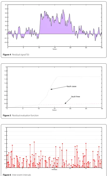
time units, and each unit length is taken ast= 5 s. The jumping modes path from time step 0 to time step 30, the switching modes path is chosen according to the ADTτa> 8.7091 constraint, which are shown in Figs. 2 and 3, respectively. Further, the residual evaluation function are shown in Figs. 4 and 5, which means the fault is detected. From Fig. 4, we know that if we enlarge the parametersDf1,Df2, the effect of fault on the outputy(t) will

be larger, so the residual signalˆr(t) becomes larger, and the detection time of fault will be reduced. Based on our results, we can obtainJth=suph(t) =0

f(t)=0

E(₃₀1 ₀30rˆT_{(t)rˆ(t)dt) = 0.1220}

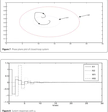
and Fig. 5 show us that (_10.021 ₀10.02ˆrT_{(t)ˆr(t)dt) = 0.2037 >Jth, that is fault signal will be} detected after 0.02 s. Meantime, Fig. 6 shows the inter-event intervals, obviously, from Fig. 6, we can know that the event is triggered 145 times during the simulation time period. Finally, the phase plane plot of the closed-loop system is shown in Figs. 7 and 8 depicts that the states of the system (10) is stability in finite time with our proposed control strategy in this paper.

5 Conclusions

Figure 4Residual signalˆr(t)

Figure 5Residual evaluation function

Figure 7Phase plane plot of closed-loop system

Figure 8System responses withut

switching has been investigated. A mode-dependent detector/controller are designed, which guarantees the closed-loop system is SSFTS and satisfies fourH∞performance

in-dices. By using some novel integral inequalities and the optimization technique, the results are derived in terms of the LMIs. Finally, a numerical example is provided to illustrate the effectiveness of the proposed method.

Acknowledgements

All authors are grateful to the anonymous referees for several comments and suggestions of improvement. This work was supported in part by the National Natural Science Foundation of China under Grants 11661028, 11661030, 11502057, the Natural Science Foundation of Guangxi under Grant 2015GXNSFBA139005, 2014GXNSFBA118023. This work was also supported by the China Scholarship Council (201608455012).

Competing interests

All the authors declare that they have no competing interests.

Authors’ contributions

All three authors contributed equally to this work. They all read and approved the final version of the manuscript.

Author details

1_{College of Science, Guilin University of Technology, Guilin, P.R. China.}2_{School of Mathematical Sciences, University of}

Electronic Science and Technology of China, Chengdu, P.R. China.3_{School of Science, Hubei University for Nationalities,}

Publisher’s Note

Springer Nature remains neutral with regard to jurisdictional claims in published maps and institutional affiliations.

Received: 17 November 2017 Accepted: 20 February 2018

References

1. Gao, H., Chen, T., Wang, L.: Robust fault detection with missing measurements. Int. J. Control81, 804–819 (2008) 2. Luo, M., Zhong, S.: Robust fault detection of uncertain time-delay Markovian jump systems with different system

modes. Circuits Syst. Signal Process.33, 115–139 (2014)

3. Liu, J., Yue, D.: Event-triggering in networked systems with probabilistic sensor and actuator faults. Inf. Sci.240, 145–160 (2013)

4. Dong, H., Wang, Z., Gao, H.: Fault detection for Markovian jump systems with sensor saturations and randomly varying nonlinearities. IEEE Trans. Circuits Syst. I, Regul. Pap.59, 2354–2362 (2012)

5. Hwang, I., Kim, S., Kim, Y., Seah, C.E.: A survey of fault detection, isolation, and reconfiguration methods. IEEE Trans. Control Syst. Technol.18, 636–653 (2010)

6. Jiang, B., Staroswiecki, M., Cocquempot, V.:H∞fault detection filter design for linear discrete-time systems with multiple time delays. Int. J. Syst. Sci.34, 365–373 (2003)

7. Wan, X., Fang, H.: Fault detection for discrete-time networked nonlinear systems with incomplete measurements. Int. J. Syst. Sci.44, 2068–2081 (2013)

8. Shokouhi-Nejad, H., Rikhtehgar Ghiasi, A., Badamchizadeh, M.A.: Robust simultaneous finite-time control and fault detection for uncertain linear switched systems with time-varying delay. IET Control Theory Appl.11, 1041–1052 (2017)

9. Zhong, G., Yang, G.: Robust control and fault detection for continuous-time switched systems subject to a dwell constraint. Int. J. Robust Nonlinear Control25, 3799–3817 (2015)

10. Zhai, D., Lu, A., Li, J., Zhang, Q.: Simultaneous fault detection and control for switched linear systems with mode-dependent average dwell-time. Appl. Math. Comput.272, 767–792 (2016)

11. Li, J., Park, J.H., Ye, D.: Simultaneous fault detection and control design for switched systems with two quantized signals. ISA Trans.66, 296–309 (2017)

12. Shokouhi-Nejad, H., Rikhtehara Ghiasi, A., Badamchizadeh, M.A.: Robust simultaneous fault detection and control for class of nonlinear stochastic switched delay systems under asynchronous switching. J. Franklin Inst. (2017). https://doi.org/10.1016/j.jfranklin.2017.05.037

13. Wang, H., Yang, G.: Simultaneous fault detection and control for uncertain linear discrete-time systems. IET Control Theory Appl.3, 583–594 (2009)

14. Davoodi, M.R., Golabi, A., Talebi, H.A., Momeni, H.R.: Simultaneous fault detection and control design for switched linear systems based on dynamic observer. Optim. Control Appl. Methods34, 35–52 (2013)

15. Marcos, A., Balas, G.J.: A robust integrated controller/diagnosis aircraft application. Int. J. Robust Nonlinear Control15, 531–551 (2005)

16. Li, T., Fu, J.: Event-triggered control of switched linear systems. J. Franklin Inst. (2017). https://doi.org/10.1016/j.jfranklin.2017.05.018

17. Shen, H., Su, L., Wu, Z., Park, J.H.: Reliable dissipative control for Markov jump systems using an event-triggered sampling information scheme. Nonlinear Anal. Hybrid Syst.25, 41–59 (2017)

18. Wang, Y., Lim, C., Shi, P.: Adaptively adjusted event-triggering mechanism on fault detection for networked control systems. IEEE Trans. Cybern.47, 2299–2311 (2017)

19. Shi, P., Wang, H., Lim, C.: Network-based event-triggered control for singular systems with quantizations. IEEE Trans. Ind. Electron.63, 1230–1238 (2016)

20. Wang, Y., Shi, P., Lim, C., Liu, Y.: Event-triggered fault detection filter design for a continuous-time networked control system. IEEE Trans. Cybern.46, 3414–3426 (2016)

21. Yue, D., Tian, E., Han, Q.: A delay system method for designing event-triggered controllers of networked control systems. IEEE Trans. Autom. Control58, 475–481 (2013)

22. Amato, F., Ariola, M., Cosentino, C.: Finite-time stability of linear time-varying system: analysis and controller design. IEEE Trans. Autom. Control55, 1003–1008 (2010)

23. Amato, F., Ariola, M., Cosentino, C.: Finite-time stabilization via dynamic output feedback. Automatica42, 337–342 (2006)

24. Chen, J., Xiong, L., Wang, B., Yang, J.: Robust finite-time boundedness ofH_∞filtering for switched systems with time-varying dely. Optim. Control Appl. Methods37, 259–278 (2016)

25. Wen, J., Nguang, S.K., Shi, P., Peng, L.: Finite-time stabilization of Markovian jump delay systems-a switching control approach. Int. J. Robust Nonlinear Control27, 298–318 (2017)

26. He, S., Liu, F.: Finite-timeH∞fuzzy control of nonlinear jump systems with time-delays via dynamic observer-based state feedback. IEEE Trans. Fuzzy Syst.20, 605–614 (2012)

27. Wu, Y., Cao, J., Li, Q., Alsaedi, A., Alsaadi, F.E.: Finite-time synchronization of uncertain coupled switched neural networks under asynchronous switching. Neural Netw.85, 128–139 (2017)

28. Lewis, F.L.: A survey of linear singular systems. Circuits Syst. Signal Process.22, 3–36 (2007)

29. Zhao, Y., Zhang, W.: New results on stability of singular stochastic Markov jump systems with state-dependent noise. Int. J. Robust Nonlinear Control (2015). https://doi.org/10.1002/rnc.3401

30. Fu, L., Ma, Y.: Passive control for singular time-vary system with actuator saturation. Appl. Math. Comput.289, 181–193 (2016)

31. Ma, Y., Yang, P., Yan, Y., Zhang, Q.: Robust observer-based passive control for uncertain singular time-delay systems subject to actuator saturation. ISA Trans.67, 9–18 (2017)

32. Zhao, X., Zhang, L., Shi, P., Liu, M.: Stability of switched positive linear systems with average dwell time switching. Automatica48, 1132–1137 (2012)

34. Liu, X., Yu, X., Zhou, X., Xi, H.: Finite-timeH_∞control for linear systems with semi-Markovian switching. Nonlinear Dyn. 85, 2297–2308 (2016)

35. Yang, B., Wang, J., Wang, J.: Stability analysis of the delayed neural networks via a new integral inequality. Neural Netw.88, 49–57 (2017)