R E S E A R C H
Open Access
Analyzing the performance of Aloha in string
multi-hop underwater acoustic sensor networks
Hongyang Yu, Nianmin Yao
*, Shaobin Cai and Qilong Han
Abstract
In this article, we intend to investigate the performance of channel access protocols in multi-hop underwater acoustic sensor networks, which are characterized by long propagation delays and limited channel bandwidth. An analytical model specifically designed for contention-based protocols in multi-hop underwater acoustic networks is identified and validated. The model is based on an underwater network model, called string topology network model, which provides a method for computing the expected network throughput and the probability of packets’ delivery to the gateway from an arbitrary sensor. This study demonstrates an improvement of an existing model, in which a node is implicitly assumed to be able to transmit two packets at the same time, which is not realistic due to the half-duplex character of underwater acoustic channels. Based on our findings, we propose a modified analytical model and evaluate it using NS-3 simulator. Results show that our analytical model is more precise than the existing one.
Keywords:Underwater acoustic sensor networks, Performance analysis, Medium access control (MAC) protocol,
Aloha, Multi-hop
Introduction
Underwater sensor networks are becoming an important research topic. They enable a wide range of collaborative applications, such as navy military surveillance, oceano-graphic data collection, ocean resource exploration, dis-aster prevention, and so on. Since both radio and optical signals suffer significant attenuation in salty water [1], acoustic technology is the typical physical layer commu-nication method adopted by the underwater sensor net-works, namely, underwater acoustic sensor networks (UASNs). However, the speed of acoustic waves in water is only approximately 1500 m/s, which is five orders of magnitude lower than the radio propagation speed. And the bandwidth of acoustic channels in water is one-thousandth that of the radio channels. Thus, compared with wireless sensor networks (WSNs), the research on UASNs is featured by long propagation delay and limited bandwidth, which pose grand challenges to almost every layer of network protocol stack and applications [2-8].
Similar to the WSNs, medium access control (MAC) protocols play a very important role in UASNs, which has
high impact on the performance of the networks. Cur-rently, theoretical analyses regarding MAC methods for UASNs focus on single-hop topology, which are summa-rized in surveys [5,9]. In particular, Xie and Cui [6] presented some theoretical analyses of contention-based protocols such as Aloha for UASNs. However, in reality, multi-hop network is more practical and it can provide wider coverage [10]. Therefore, in this article we focus on the study of multi-hop underwater scenarios.
Pure Aloha is one of the contention-based MAC proto-cols, which allows nodes to transmit whenever it is needed. And Aloha has become the basis of many wireless MACs since its proposal in the 1970s [11]. Due to the long propagation delay and limited bandwidth of acoustic channels, contention-based protocols tend to be effective for multi-hop UASNs [12].
In [7], the first analytical model is proposed for the contention-based protocols in string multi-hop networks, called string topology network model (STNM). The model provides a method for computing the expected network throughput and the probability of packets’ delivery to the gateway from an arbitrary sensor. As a follow-up work, the performance of p-persistent Aloha is analyzed in [13]. In addition, a summary of these models are provided in [14]. * Correspondence:[email protected]
College of Computer Science and Technology, Harbin Engineering University, Harbin, China
In fact, the analytical model in [7] is questionable in three aspects. First, since the node cannot transmit two packets simultaneously, there is no collision among the packets sent by the same node. However, the analytical model includes the corresponding probability, and thus the collision probability of a packet reception must be higher than the actual one. Second, the packet transmit-ting rate is equal to the aggregate traffic rate of the same node in the analytical model. But in fact the former should be less than the latter, since the generated packet will be dropped when the node is sending packet. Third, the analytical model is not validated by the simulations or experiments, which make it less convincing.
In this article, we propose a modified analytical model of Aloha protocol for string multi-hop UASNs. In order to validate the new analytical model, we simulate Aloha protocol in a string multi-hop network via NS-3. A com-parison between STNM and our analytical model is done. The results show that the analytical results obtained from our analytical model are more accurate than the ones obtained from STNM. Besides, based on our analytical model, we derive expressions for the system throughput and average end-to-end packet delay.
The remainder of this article is organized as follows. Section Performance analysis of multi-hop Aloha gives a brief overview of the string topology network, and iden-tifies the modified analytical model of Aloha for string multi-hop UASNs. Section Experiments validates our model via simulations and analyzes the differences between the results obtained from our analytical model and the simulation results. Finally, Section Conclusion concludes the study.
Performance analysis of multi-hop Aloha
In this section, we first briefly describe the string topology network [11]. Based on the string multi-hop topology, we then present an analytical model of Aloha protocol in string multi-hop UASNs. After that, we consider the ana-lytical model in another way, and prove that the two
models are equivalent. At the end of this section, the per-formance expressions for string multi-hop UASNs are de-rived from our model.
String topology network
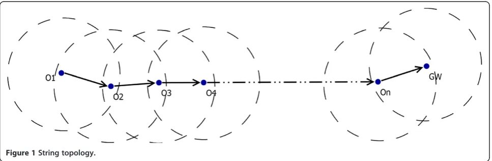
Same as in [7], in our analytical model we adopt the string multi-hop topology as depicted in Figure 1. In the string topology network, each node generates packets following Poisson distribution with generating rate λ, i.e., on aver-age, each node generatesλpackets per second. Each node immediately forwards the packet received from its up-stream neighbor to its downup-stream neighbor. And the transmission range of each node is assumed to be only capable to reach its 1-hop neighbors and the interference range is less than the distance to any 2-hop neighbor. In this article, we only consider packet loss caused by colli-sions. We also assume that all packets in collisions will get lost, since the differences of signal strength between packets involved in the collision are not large enough. It is further assumed a fixed packet size and uniform transmis-sion rate for all nodes, which result in a constant packet transmission timeT.
We notice the fact that a generated packet cannot be transmitted when the node is busy with sending. Our analytical model considers this while it is ignored by STNM. A packet sent out by each node may not follow a Poisson distribution since a packet may not be trans-mitted. In simulation, the packet will be dropped when it cannot be transmitted. As a result, the packet transmit rate is less than the aggregate traffic rate for each node.
As mentioned in [7], the string topology shown in Figure 1 favors the downstream traffic over the upstream traffic in underwater acoustic channels, as the packet from the downstream will be dropped only if it collides with other packets at a node further downstream.
Improved analytical model
In order to analyze the performance of Aloha for UASNs, we need to address the success rate of packet reception at
each hop. Letλidenote the aggregate traffic rate for node Oi. The success probability ofOi’s transmission, Pi, is the success probability that Oi+1receives its packet, which is
given as below [7]:
Pi¼Prfsuccessful reception at Oiþ1jpacket transmitted by Oig
ð1Þ
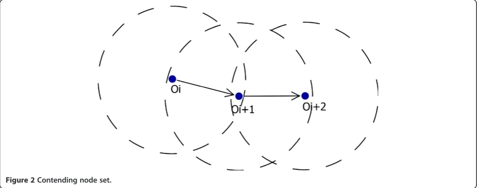
The original model (STNM) in [7] determines the like-lihood that any node in the contending node set Ci = {Oi, Oi+1, Oi+2} will inject traffic such that it arrives at
the reception point at any time during the reception of the packet of interest, as depicted in Figure 2. Based on the results, the model derives a series of equations relat-ingPitoλi,i=1,. . .,n.
However, there are three disadvantages in STNM. First, the packet transmitting rate of Oiis equal to λi in STNM. But in fact the former is less than the latter, be-cause some packets may not be sent out. Second, we consider the reception of a packet fromOiat node Oi+1.
The duration thatOi takes to transmit a packet is equal to the duration Oi+1 takes to receive the packet in
STNM. Due to Oi cannot transmit two packets at the same time, there should be no collision atOi+1between
the packets fromOi. That is, the probability of successful reception has nothing to do with whether or not Oi is sending packets whenOi+1is receiving a packet fromOi. Therefore, in STNM, the collision probability of a packet reception must be higher than the actual one, since the model includes the corresponding probability. At last, STNM is not validated by the simulations or experiments.
Before going further, let us denote the actual transmit rate of Oias λtransmit(i), and the successful transmission
probability of a packet fromOiasPtransmit(i). The
send-ing of a packet fromOican be done if and only if Oiis not sending at that moment. Hence, the probability that a packet can be sent out byOiis equal to the probability
that no traffic is generated by Oi in one packet’s trans-mission time, i.e.,T. Recalling that the packet generation of each node follows a Poisson distribution, we have
Ptransmitð Þ ¼i e
The aggregate traffic for node Oi+1includes the traffic
received from Oi and the one generated by Oi+1. Given
that each node originates packets at the same rate, we have
Furthermore, the actual transmit rate for each node is
λtransmitð Þ ¼i λi⋅Ptransmitð Þi
¼ f λeλT i¼1
λtransmitði1ÞPi1þλ
ð Þ⋅eðλtransmitði1Þ⋅Pi1þλÞT i¼2;. . .;n ð5Þ
The successful reception of a packet from Oi at node Oi+1 depends on the state of Oi+1. The reception of a
packet will fail while Oi+1 is currently overhearing the
transmission of a packet by its downstream neighbor
Oi+2, or currently sending a packet to Oi+2. And the
reception of a packet will succeed only if Oi+1is idle in
twice the packet’s reception time, i.e., 2T. These con-straints are independent.
Since the packets’arrival at node follows the Poisson process, the probability that no traffic is sent out by Oj is equal to the probability that no traffic arrives at Oj.
The probability that no packet is sent out byOjduring a packet’s reception period is
eλjð2TÞ⋅ λ jð2TÞ
0
0! ¼e
λjð2TÞ ð6Þ
Therefore, the probability of a successful reception of a packet fromOiis
Pi¼eðλtransmitðiþ1Þþλtransmitðiþ2ÞÞð2TÞ;i¼1;. . .n2 Pn1¼eλtransmitð Þnð2TÞ
Pn¼1
ð7Þ
Combining Equations (5) and (7), we can obtain nonlinear equations with respect to n variables: λtransmit
(1),λtransmit(2) ,. . .,λtransmit(n). This can be achieved by
solving the following minimization problem
minλtransmitð Þ1;λtransmitð Þ2;...;λtransmitð Þn
Xn
i¼1
Fi0ð Þ Λ λtransmitð Þi
h i2
ð8Þ
where Λ= (λtransmit(1) λtransmit(2). . .λtransmit(n)), and Fi0ð ÞΛ is calculated by iterative computation using Equation (5).
The Nelder-Mead simplex method has been quite ef-fective to solve the above minimization problems [15]. In Section Experiments, we will calculate above equa-tions and obtain the analytical results using this method in Matlab.
Equivalent modification analytical model
Reconsidering the situation where the packet is gener-ated when some packet is being transmitted. In this situ-ation, the packet will be dropped, since it cannot be transmitted. We suppose this situation as a collision, though in this case there is no collision occurs actually. We term this situation as“drop collision,” and we term the collision which occurs actually as “usual collision.” However, there is a difference between drop collision and usual collision. In drop collision, the packet which is being transmitted will not be lost. However, all packets will be lost in usual collision. Let Psuccess (i) denote the
Table 1 Parameter setting
Parameter Value
Transmission time 1 s
Data rate 256 bps
Packet size 32 Bytes
Total node number 9
Channel bandwidth 10–14 kHz
Transmit power 190 dB re 1 uPα
Minimum SIR 10 dB
Simulation time 20,000 s
The position of each node (45,000i, 0, 100)
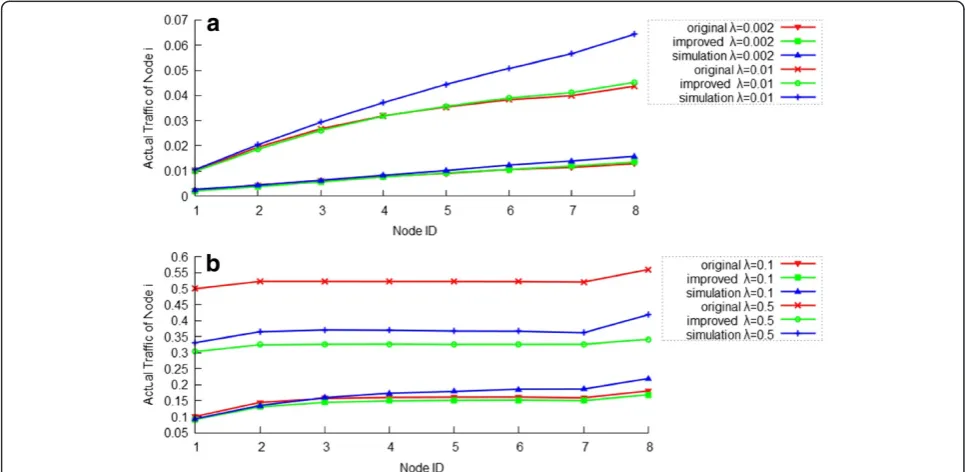
Figure 3Original, improved, and simulation results of node actual traffic load (λtransmit(i)) versus node ID atλ= 0.002, 0.01, 0.1,
success probability that Oi+1 receives the packet arrived
atOi. More formally stated, that is
Psuccessð Þ ¼i Prfsuccessful reception at Oiþ1jpacket arrived at Oig
ð9Þ
and others are same as above. Therefore, we have
λ1¼λ
λi¼λi1⋅Psuccessði1Þ þλ¼λ⋅ 1þ
Xi1
j¼1 Yi1
k¼j
Psuccessð Þk !
;
i¼2;. . .;n ð10Þ
Following these definitions, the successful reception of a packet fromOiat nodeOi+1depends on the state ofOi andOi+1. The reception of a packet fromOiis successful only if Oi is not sending some packet and no other packets arrive at Oi+1 during one packet’s reception
period. In other words, there are three possible reasons for a packet from Oito get lost: first, the packet gener-ated by Oi is tried to be sent when Oi is transmitting some other packet; second, the packet arrives at Oi+1
when Oi+1 is currently overhearing a packet from Oi+2
or Oi+1 is transmitting some packet to Oi+2; and third, Oi+1 initiates a transmission or some packet from Oi+2
arrives atOi+1whenOi+1is receiving the packet.
There-fore, the reception success probability atOi+1is
Psuccessð Þi ¼eðλiþ1⋅Ptransmitðiþ1Þþλiþ2⋅Ptransmitðiþ2ÞÞ⋅ð2TÞλiT
¼eðλtransmitðiþ1Þþλtransmitðiþ2ÞÞ⋅ð2TÞλiT
;i¼1;. . .;n2
¼Pi⋅Ptransmitð Þi
Psuccessðn1Þ ¼eðλn⋅Ptransmitð ÞnÞ⋅ð2TÞλn1T
¼eλtransmitð Þnð2TÞλn1T¼P
n1⋅Ptransmitðn1Þ
Psuccessð Þn ¼eλnT ¼1Ptransmitð Þ ¼n Pn⋅Ptransmitð Þn
ð11Þ
Combining Equations (10) and (11), we have
λ1 ¼λ
¼λi1⋅Psuccessði1Þ þλ
λi ¼λi1⋅Pi1⋅Ptransmitði1Þ þλ ;i¼2;. . .;n
¼λtransmitði1Þ⋅Pi1þλ
ð12Þ
We can see that this analytical model is equivalent to the one described in Section Improved analytical model.
Network performance expressions
LetUi denote the utilization of the link fromOito Oi+1.
The utilization of the network and the effective
throughput of the sensor network, denoted by U(n) and
S(n), can be expressed as follows
U nð Þ ¼Un¼λtransmitð Þn ⋅Pn
S nð Þ ¼λtransmitð Þn ⋅Pn⋅L⋅α ð 13Þ
where λtransmit (n) and Pn are calculated by Equations (5), (7), and (8), respectively;Lis the average packet size in bits; andαis the average fraction of data bits in each packet received by the gateway.
The end-to-end delay in networks is the sum of trans-mission and propagation delays at source and intermedi-ate nodes. The average end-to-end packet delay of the network, denoted bydelay , can be expressed as follows
delay¼X n
i¼1
Yn
j¼i Pj
! ⋅ Xn
k¼i
TþDistance ið Þ=c
ð Þ
!!
ð14Þ
wherecis the speed of acoustic waves in water;Tis the packet transmission time; and Distance(i) is the distance fromOitoOi+1.
Experiments
In this section, we first calculate the analytical results obtained from STNM (“the original results” for short) using Equations [7] and the ones obtained from our model (“the improved results”for short) using Equations (5) and (7). Then, we perform simulation with the same parameter setting using NS-3. After that, we compare STNM with the modification model, as well as validate them with the simulation results.
The NS-3 UAN module offers accurate modeling of the underwater acoustic channel and a model of the WHOI acoustic modem. Both the attenuation and noise are known to be strong functions of frequency. In our simulation, the acoustic channel model adopts Thorp at-tenuation [16], which is used for the calculation of the SNR at the receiver with the consideration of the ambi-ent noise.
Without loss of generality,T is set to be 1 s, packet size is 32 Bytes, and the simulation operation time is 20,000 s. There are nine nodes in the string multi-hop network, so nis 8. All nodes are at the same depth, 100 m. We use a channel bandwidth of 10–14 kHz, data rate of 256 bps, and transmit power of 190 dB re1 uPa. The
Figure 6The sum of the squared differences between the results obtained from the analytical model and the simulation versus theλ.
minimum SIR that the receiver requires for a correct re-ception is set to 10 dB. Thus, the packet transmission time is 32 × 8/256 = 1 s, which is equal toT. We use a path loss exponent of 1.5 corresponding to practical spreading, and absorption according to Thorp, sensor node’s communication range is between 50509 and 50510 m. We set the distance between nodes as 45000 m to make sure that a node can only talk with its one-hop neighbors. Therefore,Oi’s position is (45000i, 0, 100) in the string topology network. All parameters are listed in Table 1.
First,λis set as 0.002, 01, 0.1, and 0.5, respectively, to diversify the per-sensor load like [7]. Figure 3 shows the original, improved, and simulation results of the actual traffic load of each node (λtransmit(i), i = 1,. . ., n). Same
as claimed in [7], we can see that λtransmit(i) increases
when i increases, regardless of n. We can also observe that our improved results can better match the simula-tion results than the original ones do.
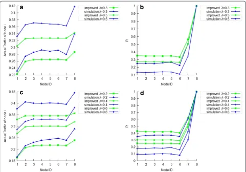
Figure 4 shows that Pi deceases except at the last two nodes due to their smaller contending node sets. When the load exceedsλ= 0.5 each node has reached its satur-ation status andPibecomes stable. In particular, no mat-ter what load is chosen, simulation results of Pn is always approaching to 1, therefore our model is more accurate than STNM.
From Figures 3 and 4, we can observe that there is still a bias between our improved results and simulation results. In order to further investigate this issue, we let λ = 0.2, 0.3, 0.4, 0.5, and 0.6, respectively. Figure 5 shows that the bias between our improved results and simulation results increases as the load goes up. One of the main reasons for the bias is that in our model and STNM, we assume that the packet transmitted by each node follows a Poisson process, which can approximately be satisfied when theλ is low. However, the interarrival time between the two ad-jacent packets transmitted is not an exponential distribu-tion, since it is more than T. Thus, with the increase of theλ, the packet transmitted by each node cannot be ap-proximately by a Poisson process any more, which con-tributes to the bias in the heavy traffic-loaded network.
In the following, we consider the sum of the squared differences between the results obtained from the analyt-ical model and the simulation. The analytanalyt-ical model which has smaller value is more accurate. Figure 6a shows the sum of the squared differences between the originalλtransmit(i) and the λtransmit(i) measured by
simu-lation, and the sum of the squared differences between the improved λtransmit(i) and theλtransmit(i) measured by
simulation versus the λ. We can observe that our im-proved results can better match the simulation results than the original ones do.
Figure 6b shows the sum of the squared differences between the original Piand the Pi measured by simula-tion, and the sum of the squared differences between the improved Pi and the Pi measured by simulation versus theλ. We can observe that our improved results are always more coincident with the simulation results than the original ones. Considering Pn significantly impacts results, we compute the sum of the squared differences of Pi except Pn, again. From Figure 6c, we can observe that the bias of our improved results still fit better than the original ones do in most cases. The above results show that our analytical model is more precise.
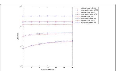
In the following, we explore the utilization of the string topology network. Gibson et al. [7] provide a method for computing the expected network utilization. Since STNM in [7] does not fit the simulation result well, we reconsider the utilization of the network using Equation (13).
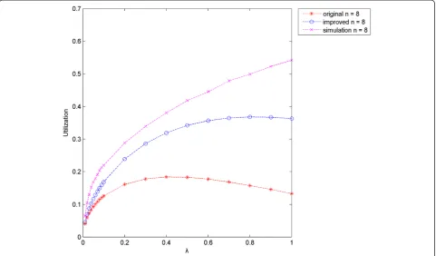
Figure 7 shows the original and improved results of utilization versus number of nodes at different load. Figure 8 shows the original, improved, and simulation results of utilization versus load, i.e., λ. As mentioned in [7], the utilization increases with n when the per-sensor load is small, since more packets arrive at the gateway when the nodes have not reached their satur-ation status. When the nodes are saturated, or almost saturated, the utilization of the network is almost flat with respect to n. However, Gibson et al.’s [7] analysis severely underestimated the utilization of Aloha in string topology UASNs, as depicted in Figures 7 and 8. The utilization can reach the maximum at about 0.3678 when the load is about 0.8. The results from STNM are less than half of the results of our model. The throughput of the network is similar with the utilization.
From Figure 8, we can also observe that the utilization obtained from our model and STNM first increases with the load. After it has reached the maximum, it starts de-creasing. However, the utilization obtained from simula-tion is monotonically non-decreasing and the maximum utilization is 1. When the load is very heavy, only the data from the last node can reach the gateway. Thus, the bias between analytical model and simulation results in-creases as the load goes up. This also indicates that the packet transmitted by each node cannot be approxi-mated by a Poisson process whenλis high.
Although there is a bias between analytical model and simulation results, our analytical model is still reason-able, sinceλ is less than 1 in most cases for underwater scenario. To further improve the analytical model’s ac-curacy, the relationship between the bias and the load should be investigated. We would like to explore this topic in our future work.
Conclusion
In this article, we identified and validated the analytical model of Aloha in multi-hop UASNs. The simulation re-sults justify that our modified analytical model is more accurate than STNM. Based on our model, we provide the expected network throughput and average end-to-end delay in string topology underwater networks.
The above analytical models are based on pure Aloha protocol which the node’s transmission has higher prior-ity than the node’s reception. It is very inefficient, since a node will simply transmit a packet whenever it has anything to send, regardless of whether it is currently re-ceiving a packet.
In the future, we would like to investigate the relation-ship between the bias and the load for our analytical model as well as further improve the accuracy of our analytical model. And we would also investigate other Aloha-based protocols such as slotted-Aloha protocol and Aloha with half-duplex protocol for string topology multi-hop network.
Competing interests
The authors declare that they have no competing interests.
Acknowledgment
This study was supported by the National Natural Science Foundation of China under Grant no. 61073047; Fundamental Research Funds for the Central Universities: HEUCFT1202 and Harbin Special funds for Technological Innovation Talents: 2012RFLXG023.
Received: 25 October 2012 Accepted: 31 January 2013 Published: 12 March 2013
References
1. F Schill, UR Zimmer, J Trumpf,Visible spectrum optical communication and distance sensing for underwater applications, in Proceedings of the Australasian Conference on Robotics and Automation, 2004
2. J Liu, Z Wang, Z Peng, J Cui, S Zhou, JSL: a joint solution for localization and time synchronization underwater sensor networks, inProceedings of the IEEE Communications Society Conference on Sensor, Mesh and Ad Hoc
Communications and Networks (SECON)(Seoul, Korea). 18–21 June 2012 3. J Liu, X Han, MA Bzoor, M Zuba, J Cui, RA Ammar, S Raj, PADP: prediction
assisted dynamic surface gateway placement for mobile underwater networks, inProceedings of the Seventeenth IEEE Symposium on Computers and Communication (ISCC’12)(Cappadocia, Turkey). 1–4 July 2012 4. J Liu, Z Wang, Z Peng, M Zuba, J Cui, S Zhou,TSMU: a time synchronization
scheme for mobile underwater sensor networks, in Proceedings of the GLOBECOM(Houston, TX, USA, 2011)
5. J Heidemann, W Ye, J Willis, AA Syed, Y Li, Research challenges and applications for underwater sensor networking, inProceedings of the IEEE Wireless Communications and Networking Conference (WCNC 2006)
(Las Vegas, NV), pp. 229–235. 3–6 April 2006
6. P Xie, J Cui, Exploring random access and handshaking in large scale underwater wireless acoustic sensor networks, inProceedings of the MTS/ IEEE Oceans Conference(Boston, 2006)
7. J Gibson, G Xie, Y Xiao, H Chen,Analyzing the performance of multi-hop underwater acoustic sensor networks, in IEEE Oceans’07(Aberdeen, Scotland, 2007)
8. J Liu, Z Zhou, Z Peng, J Cui,Mobi-Sync: efficient time synchronization for mobile underwater sensor networks, Proceedings of the GLOBECOM
(Miami, FL, USA, 2010), pp. 1–5
10. M Chitre, S Shahabudeen, M Stojanovic, Underwater acoustic
communications and networking: recent advances and future challenges. Mar. Technol. Soc. J.42, 103–116 (2008)
11. N Abramson, The ALOHA system. Proceedings of the AFIPS 1970 Fall Joint Comput Conference37, 281–285 (1970)
12. L Berkhovskikh, Y Lysanov,Fundamentals of Ocean Acoustics(Springer, New York, 1982)
13. Y Xiao, Y Zhang, JH Gibson, GG Xie, Performance analysis of p-persistent aloha for multi-hop underwater acoustic sensor networks, inInternational Conference on Embedded Software and Systems, 2009, pp. 305–311 14. Y Xiao, Y Zhang, JH Gibson, GG Xie, H Chen, Performance analysis of
ALOHA and p-persistent ALOHA for multi-hop underwater acoustic sensor networks. Cluster Comput.14, 65–80 (2011)
15. DM Olsson, LS Nelson, The Nelder-Mead simplex procedure for function minimization. Technometrics17, 45–51 (1975)
16. AF Harris, M Zorzi, Modeling the underwater acoustic channel in ns2, in
Proceedings of the 2nd international Conference on Performance Evaluation Methodologies and Tools, vol 321, Nantes, France, 22–27 October 2007
(ValueTools ICST (Institute for Computer Sciences Social-Informatics and Telecommunications Engineering), ICST, Brussels, Belgium, 2007), pp. 1–8
doi:10.1186/1687-1499-2013-65
Cite this article as:Yuet al.:Analyzing the performance of Aloha in
string multi-hop underwater acoustic sensor networks.EURASIP Journal
on Wireless Communications and Networking20132013:65.
Submit your manuscript to a
journal and benefi t from:
7Convenient online submission
7Rigorous peer review
7Immediate publication on acceptance
7Open access: articles freely available online
7High visibility within the fi eld
7Retaining the copyright to your article