ISSN: 1992-8645 www.jatit.org E-ISSN: 1817-3195
A NEW TOMOGRAPHIC BASED KEYPOINT DESCRIPTOR
USING HEURISTIC GENETIC ALGORITHM
1,2
S.HADI YAGHOUBYAN, 1MOHD AIZAINI MAAROF, 1ANAZIDA ZAINAL, 1MAHDI MAKTABDAR OGHAZ
1
Faculty of Computing, Universiti Teknologi Malaysia (UTM), Malaysia 2
Department of Computer Engineering, Islamic Azad University, Yasooj Branch, Yasooj, Iran
E-mail: 1,[email protected], [email protected], [email protected]
ABSTRACT
Keypoint descriptor is a fundamental component in many computer vision applications. Considering both computational complexity and discriminative power, SURF descriptor among non-binary and BRISK among binary descriptors are the prominent techniques in the field. Although, these descriptors have shown remarkable performance, but they are still suffering weaknesses such as lack of robustness against image transformations and distortions, especially blur, JPEG compression and lightening variation. To address this matter, a new and robust keypoint descriptor is proposed in this research which is adapted from Tomographic-Image-Reconstruction technique. Convolution of associated image patch and predefined Gaussian smoothed sensitivity maps yield a matrix whose entities demonstrate the average intensity of the pixels at the convolved pixels in the image patch. The initial descriptor vector is built by calculating the absolute differences of all possible pairs of matrix. Then, the most discriminative features of this initial descriptor vector are detected by Heuristic Genetic Algorithm (GA). The Experimental result showed that proposed keypoint descriptor outperformed some existing techniques especially in blur, JPEG compression and illumination variation while it has reasonable performance in other image transformations.
Keywords: Keypoint, Image Patch, Feature Descriptor, Tomography-Based Descriptor, Terminal Point, Genetic Algorithm, Sensitivity Map
1. INTRODUCTION
Many computer vision applications such as visual correspondence, stereo matching, image retrieval, visual recognition object tracking and many more rely on image representation with sparse number of keypoints. The existent challenge is to efficiently describe and represent the detected keypoints or image patches, with stable, robust and compact representations invariant to blur, rotation, noise, scale, and illumination or brightness change. Based on the descriptor performance evaluation for different geometric and photometric transformations [1][2][3][4] in numerous computer vision applications, considering both computational complexity and discriminative power, it can be observed that the Speeded up Robust Feature (SURF) descriptor proposed by Bay et al. [5] in non-binary descriptors and BRISK proposed by [6] in binary descriptors have better overall performance compared to other exiting techniques. However, these descriptors suffer from lack of robustness and reliability against image
transformations and distortion, in particular to blur, JPEG compression and brightness change [2][4][7].
Inspired by Tomographic-Image-Reconstruction
technique, this research proposes an adapted keypoint descriptor. A set of predefined Gaussian smoothed sensitivity maps is convolved with associated image patch which produces a matrix. Each entity of this matrix indicates the average intensity of the pixels in image patch. The initial descriptor vector is built by calculating the absolute differences of all possible pairs of matrix. The Genetic Algorithm (GA) is used to optimize initial descriptor by finding the most discriminative features.
Note that the notation interest-point, Keypoint, feature and corner refer to an anomaly point in image which could be possibly detected by feature detectors. For uniformity and consistency the notation keypoint is used throughout this paper.
ISSN: 1992-8645 www.jatit.org E-ISSN: 1817-3195 3 presents the analogy of Tomography imaging
method. The framework of the proposed technique is described in section 4. In section 5, experimental setup and evaluation of the proposed technique is presented. Finally, Section 6 concludes the paper.
2. LITERATURE REVIEW
A keypoint could be defined as a visual characteristic of the content in image. It is located in a distinct place in image which image information is prominent. This property enables the keypoint detector to detect the same keypoints under different image transformations such as change in scale, viewpoint, brightness, rotation and blur. Combination of detector/descriptor pairs considerably affect the descriptor performance. The method used in initial keypoint detection rely heavily on gradient computation such as the Harris Corner Detection [8]. Mikolajczyk & Schmid [9] have made some improvement to the Harris detector and proposed scale invariant detector. Template-based detectors are another category of keypoint detectors such as SUSAN (Smallest Univalue Segment Assimilating Nucleus) which is an early work on this category [10]. A new generation of template-based detectors introduced by [11] adapts machine learning algorithms which their detector is called FAST (Features from Accelerated Segment Test). Mair et al [12] improved the performance of FAST detector and named it AGAST (Adaptive and Generic Accelerated Segment Test) detector. Recently, the authors in binary descriptors BRISK[6] and FREAK [13] used multi-scale AGAST detector to detect keypoints. They search for maxima in scale-space using FAST score as a measure of saliency. A number of comprehensive surveys on detectors could be found in [1], [14], [15],[4], [16], [17].
Once keypoints are located by detector, we are interested in describing the image patches centered by the detected points. Usually a feature descriptor represents either a subset of the total pixels in the neighborhood of the detected keypoints or other measures generated from the keypoints and deliver a robust feature vector. Based on the literature, descriptor techniques can be categorized into two types: 1) descriptors based on geometric relations, 2) descriptors based on pixels of the interest region. In first group, the descriptors use the relationship between the keypoint locations such as the distance from, or angle of, the neighboring keypoints. Zhou et al. [18] proposed a descriptor in which a Delaunay triangle in improved version of SUSAN [10] was constructed and then the interior angles as
the properties of the descriptor were calculated. Since the interior angles of the Delaunay triangle do not change with scale or rotation transformations, their proposed descriptor is invariant to rotation and uniform scaling. Meanwhile, this descriptor is weak against non-uniform scale or affine transformations [19]. Awrangjeb and Lu [20] proposed a curvature descriptor for keypoint matching between two images. They used the information such as the keypoint location, absolute curvature values and the angle with its two neighborhood corners which is provided by their proposed CPDA [21] keypoint detector. Despite the low dimension and ease of constructing descriptors based on geometric relations, the research on this type of descriptor appears to be limited in the literature due to several weakness. First, the distinctiveness of the keypoint locations in such representation is relatively low which leads to either miss-matches or many false matches; second, this type of descriptor constantly uses the iterative process to look for the best possible matches; finally, the matching process is known to become too slow [22].
ISSN: 1992-8645 www.jatit.org E-ISSN: 1817-3195 too high. Hashing functions or Principal
Component Analysis (PCA), are used to reduce the dimensionality of these feature descriptors [29].
Recently, progress in the computer vision community has shown that a simple pixel intensity comparison test can be efficient to generate a robust binary feature descriptor. Calonder et al. [30] proposed a binary feature descriptor using a simple intensity difference test which is called BRIEF. The advantage of BRIEF descriptor is high descriptive power with low computational complexity during feature construction and matching processes. To obtain descriptor vector, intensity of 512 pairs of pixels is used after applying a Gaussian smoothing to reduce noise sensitivity. The positions of the pixels are randomly pre-selected according to Gaussian distribution around the patch center. The high matching speed is achieved by replacing usual Euclidean distance with Hamming distance (bitwise XOR followed by a bit count). The proposed descriptor is not invariant to some transformation such as rotation and scale changes unless it is coupled with detector providing it. Calonder et al. also mentioned that unnecessary orientation invariant property should be avoided because it reduces the recognition rate. Rublee et al. [31] improved BRIEF descriptor and proposed Oriented Fast and Rotated BRIEF (ORB) descriptor which is invariant to rotation and robust to noise. Similarly, Leutenegger et al. [6] proposed a scale and rotation invariant binary descriptor which is named BRISK. To build the descriptor bit-stream using a specific sampling pattern, a limited number of points are selected and Gaussian smoothing is applied to avoid aliasing effects. To build the descriptor, pairs of smoothed points is used. These pairs are divided into long-distance and short-distance subsets in which short-distance subset is used to build binary descriptor after rotating and scale normalization, the sampling pattern and the long-distance subset is used to estimate the direction of selected patch. Inspired by human visual system, Alahi et al.[13] proposed FREAK binary descriptor which uses learning strategy of ORB descriptor and DAISY-like sampling pattern [32]. A number of comprehensive surveys on detectors can be found in [1], [3], [4], [24], [33]. Despite the advantages of binary descriptors such as high performance in constructing a descriptor vector, low memory consumption and suitability for real-time and mobile-based applications, they suffer from some image transformations in terms of accuracy. In addition, the accuracy of non-binary descriptors is a challenging and complex process and requires many adjustments and considerations. To address
common descriptor problems we propose an adopted keypoint descriptor based on Tomographic image reconstruction technique.
3. ANALOGY OF TOMOGRAPHY
In this section the tomography method is briefly explained to provide the basic knowledge on proposed Tomography-Based-Descriptor. Tomography is a method of imaging a single plane, or slice, of an object resulting in a tomogram. In other words, it is the process of creating visual representations of human internal organs into image format for clinical analysis and medical intervention [34]. Conventional and computer-assisted tomography are two fundamental methods of obtaining such images. Conventional tomography employs mechanical devices to display an image directly onto X-ray film, while in computer-assisted tomography, a computer constructs a visual image of the structure which is scanned by radiation detectors. These visual images can be stored in digital format and displayed on a screen, or printed on paper or film. Imaging techniques using computer-assisted method are superior to conventional tomography. These methods are able to capture both soft and hard tissues while conventional tomography method is quite poor at imaging soft tissues[35].
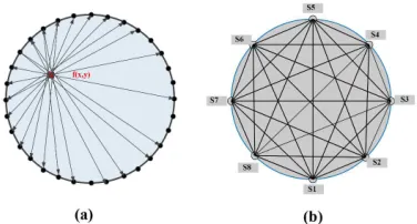
Figures 1 to 3 show the principals of tomography method and explain how to obtain the Tomographic image. Basically, the tomography imaging method consists of several sensors (Si) in a region of interest (ROI) surrounding an object which is
depicted in Figure 1. (a). An example of tomography method with 8 sensors structure and their connections are shown in Figure 1. (b).
Figure 1. The Tomography Imaging Method. A) An Example Of Tomography Structure At B) Tomography Method With 8 Sensors Structure In Which The Sensors Are Interconnected Through The Beams. The Lines In This Image Resemble The Beams Presence Of An Object.
ISSN: 1992-8645 www.jatit.org E-ISSN: 1817-3195 receiver side sensor (Figure1-a). These changes are
subject to density, size and type of an object. The number of sensors in tomography is an important parameter and it has a significant role in the reconstruction of the object’s image. In other words, the quality of reconstructed image is directly correlated to the number of sensors implemented. As the number of sensors increases, the representation of the reconstructed image will be enhanced. Figure2 illustrate an example of tomography method implementation whose an object is reconstructed by 8 and 16 sensors structure. It can be observed that 16 sensor structure generates a better reconstructed image quality compared to 8 sensor structure tomography implementation.
Figure2: Simple Demonstration Of Tomography Implementation A) Two Candidate Objects Inside The
ROI, B) Reconstructed Objects Using 8 Sensors C) Reconstructed Objects Using 16 Sensors.
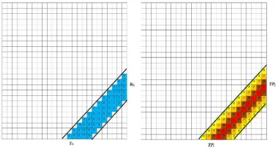
Image reconstruction consists of two stages: forward problem and inverse problem [37]. In forward problem a simulation is used to find a sensitivity map which refers to the discretized line from the transmitter’s output to the receiver’s input. On the other hand, the inverse problem is to reconstruct an image from the measured data in the forward problem. This technique is usually used to find the distribution of materials in special object. A sensitivity map is a matrix with all zero elements except the elements which are a part of a line from transmitter to receiver. Figure3 (a) shows a simple example of a sensitivity map from transmitters to receivers. Accurate forward models help to improve image reconstruction but there is no exact model to be used as reference and usually an estimated method is used. We have identified that using Gaussian smoothed sensitivity map improves the accuracy of the proposed technique. Gaussian smoothing mitigates the crosstalk effect between neighboring sensitivity maps. An example of Gaussian smoothed sensitivity map is shown in Figure3-(b). In this paper the transmitter and receiver are termed “Terminal Point”. Section 5.3 shows an example of 16 Terminal Point (TP)
Structure and all possible connections between these TPs.
Figure 3: A) Simple Sensitivity Map From Transmitter To Receiver In Tomography B) Sensitivity Map From Terminal Point I To Terminal Point J With Gaussian
Smoothing
4. METHODOLOGY
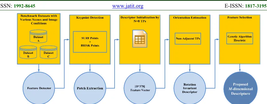
The framework of the proposed descriptor technique is depicted in Figure 4. The proposed Tomography-Based descriptor consists of five consecutive steps including Dataset, Keypoint
Detection, Descriptor Initialization (N=8),
Orientation Estimation and Feature Selection. The
following sections describes each step in more detail.
4.1 Dataset
The experimental evaluation of the proposed descriptor was performed on three different datasets. Complementary information alongside sample images of each dataset are provided:
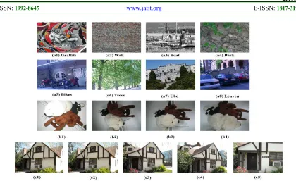
1) Mikolajczyk and Schmid (M&S): This dataset is widely used in several previous evaluation works such as [4], [6], [14]. Different photometric and geometric transformations including view-point change (Graffiti and Wall), blur (Bikes and Trees), zoom and rotation (Boat), JPEG compression (Ubc) as well as brightness changes (Leuven) are covered in the dataset. Sequence of six images are showing the increase in amount of transformation in each group. All image pairs are associated with a ground truth homography which indicates the corresponding keypoints in each image pair. The first image in each group is used as reference image in experiment [25]. Figure 5 (a1-a8) illustrates some sample images from this dataset. This dataset is publicly availableat:
ISSN: 1992-8645 www.jatit.org E-ISSN: 1817-3195
Figure 4: Framework of the proposed Tomography-Based Descriptor
2) Caltech Campus buildings(CB): The images
in Caltech Campus buildings dataset are taken from 50 buildings in Caltech university campus. For each building five different images were taken from five different angles and distances resulting in a dataset with 250 images [38]. Similar to M&S dataset, the first image in each group is used as reference image in experiment. Figure 5 (c1-c5) presents some sample images of this dataset. This dataset is
publicly available at:
http://vision.caltech.edu/malaa/datasets/calte
ch-buildings/ .
3) David Nister (DN): This dataset includes a
total of 2550 image groups taken from different scenes, object and individuals. Each image group consist of four images which were taken from different angles and distances. A subset of 100 randomly chosen image groups is utilized in our experiments.
The first image in each group is used as reference image. Figure 5 (b1-b4) illustrates some sample images of this dataset [39]. Table 1 summarizes the datasets specifications including the photometric and geometric transformations as well as number of images in each dataset. Alongside the existing transformation in dataset, this research adds Gaussian noise transformation in order to compare the descriptors performance against image noise. To carry out image noise comparison, we have manually added Gaussian noise with variance 0.05 into dataset CB and dataset DN. This dataset can be accessed online through the following website:
http://www.vis.uky.edu/~stewe/ukbench/.
Table 1: Photometric and Geometric Transformations As Well As the Number of Images In Each Dataset. Note That The Gaussian Noise Is Applied To The Images Manually.
Viewpoint Rotation Scale Brightness Blur Noise JPEG
Compression
#Image Groups
#Images per set
#Used Images Dataset
1(M&S)
× 8 6 48
Dataset 2 (CB)
× × manually
added
× 50 5 250
Dataset 3 (DN)
manually added
ISSN: 1992-8645 www.jatit.org E-ISSN: 1817-3195
Figure 5: Sample images of Mikolajczyk and Schmid (M&S) dataset (a1-a8), David Nister (DN) dataset (b1-b4) and Caltech Campus buildings (CB) dataset (c1-c5).
4.2 Keypoint Detection
The primarily step in many computer vision applications is detecting distinct locations in the image where the image information is prominent. These locations are known as keypoint. Many keypoint detectors have been presented in the literature. This paper uses the popular keypoint detectors, SURF to identify the saliency in images. These detector use the Scale-Space technique which ensures that the detected keypoints are scale invariant. For fair comparison, the number of detected keypoints in each dataset are equal for all compared descriptors.
4.3 Building Descriptor
Once the keypoints are located in the image using detector, the next step is associating every keypoint with a unique identifier or a signature which can later be used in identifying the corresponding keypoints from another image. These signatures or identifiers which are used to describe keypoints are termed descriptors. A descriptor is usually an n-dimensional vector which represents the image patch surrounding a special keypoint. In this section we describe a keypoint descriptor adapted from tomography image reconstruction technique.
In order to build an initial descriptor, we need to locate TPs in image patches using sensitivity maps. As an example Figure 6 illustrates a simple implementation of a Tomography-Based Descriptor
Technique with 16 TPs. Each TP is linked to its counterparts through a sensitivity map. The sensitivity map which we used in this research has relatively similar structure compared to sensitivity map in tomography method. The only difference is that the proposed sensitivity map uses Gaussian
normal coefficient (Figure 3. (b)) which improves
the discriminative power of feature descriptors. Eq. (1) shows the sensitivity map formula used in the proposed technique.
where is the sensitivity at position (x,y) from terminal point to terminal point , σ is standard deviation,
x
and y are the pixel center point coordinate.ISSN: 1992-8645 www.jatit.org E-ISSN: 1817-3195
where is the average pixel intensity matrix for all terminal points, is the sensitivity map from initial terminal point i ( ) to terminal point j ( ), I is the pixel intensity, N is the number of terminal points and n is the number of pixels in the sensitivity map from to .
Since the average intensity calculated from TPi to
TPj is same as the average intensity from TPj to TPi,
the inverse direction average intensity calculation is not used to create the descriptor feature vectors.
Figure 6 shows an example of 16 Terminal Point (TP) Structure and all possible connections between these TPs. Figure 6 (a) shows an example in which the terminal Point 9 (TP9) is linked to the rest of terminal points using a predefined sensitivity map. The pixel intensity average between TP9 and the rest of terminal points are calculated and recorded in a vector termed Mij where i indicates the #number
of initial terminal point and j represents the destination terminal #number. This operation will be repeated until the sensitivity map M is fully populated and all terminal points are fully linked to one another. A fully linked TPs structure is shown in Figure 6. (b).
In the next step, we construct the proposed descriptor by finding absolute differences between all possible pairs in matrix M and create
Differentiate Features Vector ‘D’. In other words,
vector D includes the difference between all possible intensity averages from TPi to TPj in the
image patch. The number of elements in the matrix M, can be computed using Eq. (3).
Note that since the average intensity is bidirectional, the inverse direction average intensity is not used to construct the descriptor feature vectors, consequently the number of elements in matrix M is divided by 2.
where K is the total number of elements in matrix M
and N is the number of terminal points. The initial feature vector of this research can be established through mathematical combination of the number of elements in matrix M as presented in Eq. (4).
Figure 6: Sample of Terminal Points in the propose technique which are linked by sensitivity map (a) linkage
between one TP to the rest of TPs (b) A fully linked TPs structure
As an example, if the number of terminal points TP in the sensitivity map is N=16, then the number of all possible intensity averages will be 120 according to equation (3), therefore the length of the feature vector D will be 14280.
In the next step, Genetic Algorithm (GA) optimization technique is used to remove redundant, correlated and noisy elements in feature vector D.
4.4 Orientation Estimation and Matching Descriptors
Non-adjacent terminal point’s (TP) location pairs which have been designated in the sensitivity map earlier are used to determine each patch orientation in an image. Sum of gradients of these pairs is used to estimate the orientation of patches. Similar to BRISK [6] the Gaussian smoothing with standard deviation σ is applied to each terminal point to mitigate aliasing effect. Suppose T be a set of all TP pairs used to compute local gradient of local image patch, the orientation of this patch can be formulated as:
ISSN: 1992-8645 www.jatit.org E-ISSN: 1817-3195
4.5 Feature Vector Optimization Using Genetic Algorithm
The presence of many highly correlated, redundant and noisy features in feature vector D degrade the accuracy of the proposed descriptor and slows down the descriptor performance. These issues need to be addressed by finding optimal feature vector subset which maximizes the discriminative power of the proposed descriptor. Considering the data type and initial feature vector dimension the Genetic Algorithm (GA) is selected to be used in this study because it shows relatively robust results compared to other optimization techniques such as greedy search, simulated annealing and evolutionary programming [39].
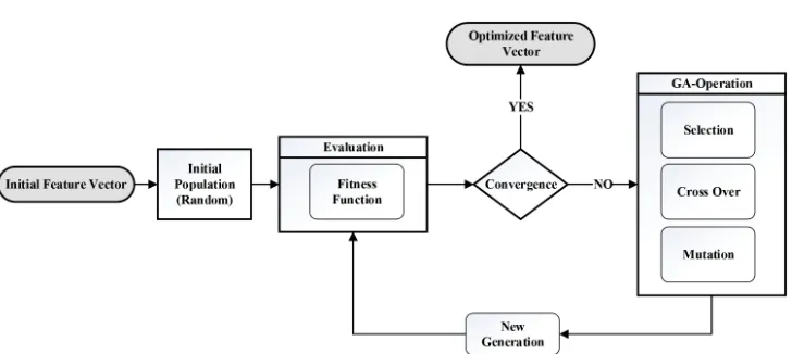
Genetic Algorithm (GA) is a technique for resolving constrained and unconstrained optimization problems according to a natural selection process that imitates the biological evolution. Figure 7 presents the block diagrams of finding optimal feature vector using Genetic Algorithm.
To reduce the computational complexity, our experiment used 8 terminal points (TP) in the sensitivity map. Applying Eq. (3) and (4), the 8 terminal points generated initial feature vector D with the size of 378 elements.
Initial population size which is incrementally generated is comprised of feature vector subsets (candidate optimal solutions) each consisting of a random set of features (average intensity differences). Random generation of initial population allows the entire search space to contribute in the formation of an optimal solution. Proper population size is very dependent on the nature of the problem. In this experiment, we have measured the cost value of the Genetic Algorithm with different population sizes ranging from 10 to 60 in order to determine the right population size. The experiment shows that population size of 40 is the best where GA solution delivers an optimum descriptor (Figure 8 (a)). The GA is frequently trapped in local maxima at population sizes smaller than 40, while population sizes larger than 40 only increase the computational complexity of the operations; however they nearly converged to the identical solution. Figure 8 (b) illustrates the cost of the candidate solutions across different feature vector sizes ranging from 5 to 375 features. According to Figure 8 (b) feature vector with size of 190 generates optimal results. Thus, the best proposed descriptor length in this experiment is 190.
ISSN: 1992-8645 www.jatit.org E-ISSN: 1817-3195
Figure 8. a) Average Cost value of the GA optimized feature vector under different population sizes ranging
from 10 to 60 individuals b) Cost value of genetic algorithm optimal solution under different feature vector
sizes ranging from 5 to 375 individuals.
An appropriate cost function is vital for proper application of Genetic Algorithm. In this experiment the cost function is aimed at minimizing the ratio between feature vector distances which are wrongly matched to correctly matched feature vector distances. Eq. (6) shows the proposed cost function.
1 2
1
1 2
1
/
/
N
F i F i i
N
C i C i i
D
D
N
Cost Function
D
D
N
= =
−
=
−
∑
∑
(6)where and are i-th element in the two feature vector which are correctly matched , and are i-th element in the two feature vector which are wrongly matched and N is the number of elements in the feature vector D.
After each iteration, individuals with higher cost values will be selected to partially reproduce next generation's population. In order to generate the successive generations, Bayesian optimization algorithm (BOA) is applied. The GA iterates until a termination condition is met. The maximum number of iterations is experimentally fixed to 400 generations.
Crossover and mutation are two main Genetic Algorithm operations. Crossover indicates how the genetic algorithm forms a crossover child for the next generation by combining two individuals, or
parents. The other GA operation is mutation which is responsible for making small random changes in the individuals in the population to create mutant children. Mutation enables the Genetic Algorithm to search for a broader space and provides genetic diversity. Mutation is also aimed to avoid the population of chromosomes from becoming too similar to other populations, and allows the GA to prevent local minima.
5. EXPERIMENTAL SETUP AND EVALUATION
This section presents qualitative and quantitative evaluation results of the proposed
Tomography-Based Descriptor technique. It also presents a
comparison between the proposed technique and several state-of-the art image descriptors including the well-known SURF descriptor and several recent binary descriptors such as BRISK and FREAK descriptors. The proposed descriptor is created using only 8 terminal points. Increasing the number of terminal points can possibly result in higher discriminative power and performance. In GA parameter setting, based on assumptions in [40] the Mutation and crossover probabilities were set to 0.025 and 0.4 respectively. Meanwhile, the population size is fixed to 40 which is obtained experimentally and maximum number of iterations is set to 400 generations. This section begins with a short description on evaluation metrics of this research and concludes with the experimental results and analysis.
5.1 Evaluation Metrics
The following evaluation metrics in Eq. (7) and Eq. (8) which are proposed by [24] are used in this work to evaluate and compare the performance of the proposed Tomography-Based descriptor technique with some representative state-of-the art techniques. These metrics are defined as follows:
ISSN: 1992-8645 www.jatit.org E-ISSN: 1817-3195 estimated by computing the feature
correspondences between pairs of images followed by the state-of-the-art RANSAC implementation USAC [41]. To compute feature correspondence, a brute force nearest neighbor algorithm is used to find the best potential matches in the second image for each feature in the first image.
The other evaluation metrics used are Correct Matches Rate (CMR) which is the percentage of correct matches (CM) to total matches(TM) and False Matches Rate (FMR) which is the percentage of false matches (FM) to total matches(TM). These parameters which are similar to Precision and Recall are used in Caltech Campus and David Nister datasets. The difference is that here we compared the percentage of correct matches to total matches of whole dataset. CMR and FMR are formulated as follows:
5.2 Result and Analysis
The proposed descriptor has been evaluated using some established evaluation technique and datasets. In the first dataset which is proposed by [24], Precision-Recall curve using threshold-based similarity matching is used to evaluate the performance of the proposed descriptor. Unlike the nearest neighbor matching technique, which looks up for matches with the lowest descriptor distance in a dataset, the similarity matching technique pair of keypoints is assumed matched if the descriptor distance is below a certain threshold value. Figure 9 shows the Precision-Recall curves of Mikolajczyk and Schmid datasets over transformations such as view point, blur, brightness, JPEG compression, rotation and scale change. SURF, BRISK and FREAK descriptors are used for comparison.
Note that (SURF detector) was used for all descriptors in first experiment. For benchmarking purpose, we have used the same descriptor parameter used by many researchers [5], [6], [13]. In terms of blur transformation Figure 9 shows that proposed descriptor has relatively superior performance compared to other descriptors. In addition, the proposed method BRISK descriptor also shows relatively promising performance. Surprisingly, FREAK descriptor shows relatively poor performance in terms of blur transformation in
this dataset. It seems that this descriptor is not suited to the threshold test which is reported in [3] as well. This is probably due to distribution of distances seen in practice.
In terms of brightness transformation, in lower descriptor distance thresholds, BRISK and FREAK descriptors have better performance. However, as we increase the threshold value, these techniques left behind the proposed descriptor. Surf descriptor has the worst performance in brightness transformation. With regard to JPEG compression, in majority of threshold domain, the proposed descriptor has superior performance compared to other descriptors. BRISK descriptor also has relatively good performance in this experiment. Similar to blur transformation, FREAK descriptor delivers relatively poor performance. In terms of view point transformation, BRISK descriptor has the highest performance compared to other descriptors in this experiment.
Figure 9: The Quantitative Evaluation Of Proposed Descriptor Compare To SURF, BRISK And FREAK
Descriptors Over Dataset 1.
ISSN: 1992-8645 www.jatit.org E-ISSN: 1817-3195 FREAK descriptors have superior performance
among the descriptors in the experiment. The results reported in [3] also support our experimental results. Generally, the performance of descriptor cannot be properly judged based on only a particular dataset, because the pair’s rank and rates might change considerably in different scenes and image types in the real word.
The second evaluation environment is performed on dataset 2 and dataset 3. Table 2 and 3 show the average false match and correct match rates of different descriptors over all images in Caltech Campus Building Database (CB) and David Nister dataset (DN) respectively. In these experiments image one of each image group (reference image) is probed with other images in each image group to find the potential match descriptors. Unlike the experiments in Figure 9 these experiments use different detectors which are SURF and BRISK detectors to detect keypoints in image. For fair comparison the detectors are tuned such a way that number of detected features are almost equal for both detectors.
Based on table 2, SURF-SURF detector/ descriptor pair with CMR=67.5% and CMR=64% in image pairs 1-2 and 1-3 respectively delivers
better performance compared to other detector/descriptor pairs in this experiment. However, for image pair 1-5 the combination of SURF detector and the proposed descriptor with
CMR=65.5% outperforms the other
detector/descriptor pairs. Table 2 also shows that BRISK-FREAK pair has relatively poor performance in this dataset.
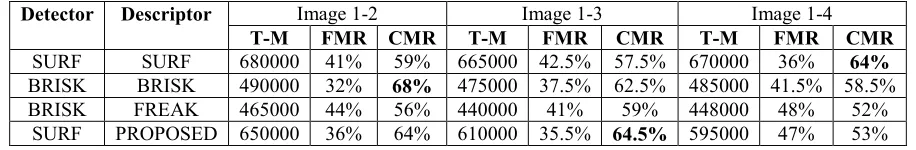
Table 3 shows the average false matches and correct matches of David Nister Dataset. The table shows that BRISK-BRISK detector/descriptor pair with CMR=68% in image pairs 1-2 delivers better performance compared to other detector/descriptor pairs in this dataset. In image pair 1-3, the proposed descriptor with CMR=64.5% has superior performance compared to other descriptors. Finally, SURF-SURF pair which generates the CMR=64% has relatively better performance in image pair 1-4. According to Figure 9 and tables 1 and 2 we can conclude that the proposed Tomography-Based descriptor has the edge in blur, brightness and JPEG compression transformation. Meanwhile, it has reasonable performance in view point, rotation and scale transformations. Note that the performance of descriptors is very dependent on the combination of detector/descriptor pairs and the dataset.
Table 2. Detector/descriptor pair performance evaluation for Caltech Campus Building Database. TM = the total number of matches over whole dataset, FMR = the percentage of False Matches and CMR = the percentage of Correct
Matches.
Detector Descriptor Image 1-2 Image 1-3 Image 1-5
TM FMR CMR TM FMR CMR TM FMR CMR
SURF SURF 510000 32.5% 67.5% 480000 36% 64% 450000 48% 52%
BRISK BRISK 260000 55% 45% 210000 51.5% 48.5% 200000 45.5% 44.5%
BRISK FREAK 248000 64.5% 35.5% 195000 58% 42% 180000 49% 51%
SURF PROPOSED 445000 51% 49% 350000 39.5% 60.5% 290000 43.5% 56.5%
Table 3. Detector/descriptor pair performance evaluation for David Nister Database.
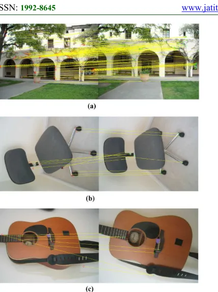
In order to demonstrate the proposed descriptor performance in addition to the quantitative evaluations provided above, qualitative evaluation of proposed descriptor is depicted in Figure10. Several image pair samples are randomly selected from datasets 2 and 3. These image pairs consist of
various transformations mentioned in table 1. The yellow color lines which link the detected keypoints in each image pair shows the total descriptor matches in the proposed descriptor. However we can observe few false matches in some cases.
Detector Descriptor Image 1-2 Image 1-3 Image 1-4
T-M FMR CMR T-M FMR CMR T-M FMR CMR
SURF SURF 680000 41% 59% 665000 42.5% 57.5% 670000 36% 64%
BRISK BRISK 490000 32% 68% 475000 37.5% 62.5% 485000 41.5% 58.5%
BRISK FREAK 465000 44% 56% 440000 41% 59% 448000 48% 52%
ISSN: 1992-8645 www.jatit.org E-ISSN: 1817-3195
Figure 1: The qualitative evaluation of the proposed descriptor over datasets 2 and 3.
6. CONCLUSION
In this study we have proposed keypoint descriptor based on Tomographic Image Reconstruction using heuristic Genetic Algorithm. A predefined Gaussian smoothed sensitivity map together with Genetic Algorithm (GA) were used to generate the proposed descriptor. The proposed Tomography-Based descriptor was evaluated using three benchmark datasets in [24] [37] [38]. The main findings of this study demonstrate that the proposed Tomography-Based descriptor outperforms representative state-of-the art techniques in image distortions and transformations in particular blur, brightness and JPEG compression. Meanwhile, it has reasonable performance in view point, rotation and scale transformations. Note that the performance of descriptors heavily depends on the combination of detector/descriptor pairs and the dataset. The proposed descriptor can be applied in many different computer vision and image retrieval applications such as low quality medical images.
7. ACKNOWLEDGEMENT
The research is funded by Universiti Teknologi Malaysia’s Research University Grant (PY/2014/02479).
8. REFERENCES
[1] O. Miksik and K. Mikolajczyk, “Evaluation of local detectors and descriptors for fast feature matching,” Pattern Recognit. (ICPR), 2012
21st …, pp. 2681–2684, 2012.
[2] J. Heinly, E. Dunn, and J. M. Frahm, “Comparative evaluation of binary features,”
Lect. Notes Comput. Sci. (including Subser.
Lect. Notes Artif. Intell. Lect. Notes
Bioinformatics), vol. 7573 LNCS, pp. 759–773,
2012.
[3] N. Khan, B. McCane, and S. Mills, “Better than SIFT?,” Mach. Vis. Appl., 2015.
[4] D. Mukherjee, Q. M. Jonathan Wu, and G. Wang, “A comparative experimental study of image feature detectors and descriptors,” Mach.
Vis. Appl., pp. 443–466, 2015.
[5] H. Bay, T. Tuytelaars, and L. Van Gool, “Surf: Speeded up robust features,” Springer berlin
Heidelberg, Comput. Vision–ECCV 2006, pp.
404–417, 2006.
[6] S. Leutenegger, M. Chli, and R. Y. Siegwart, “CV Reading BRISK : Binary Robust Invariant Scalable Keypoints,” pp. 1–8, 2011.
[7] H. Ying, J. Song, J. Wang, X. Qiu, W. Wei, and Z. Yang, “Research On Feature Points Extraction Method For Binary Multiscale And Rotation Invariant Local Feature Descriptor,”
ictactjournals.in, vol. 9102, no. August, pp.
873–878, 2014.
[8] C. Harris and M. Stephens, “A Combined Corner and Edge Detector,” Procedings Alvey
Vis. Conf. 1988, pp. 23.1–23.6, 1988.
[9] K. Mikolajczyk and C. Schmid, “Indexing based on scale invariant interest points,” Proc. Eighth IEEE Int. Conf. Comput. Vision. ICCV 2001, vol. 1, pp. 525–531, 2001.
[10] S. Smith and J. Brady, “SUSAN—a new approach to low level image processing,” Int. J.
Comput. Vis., vol. 23, no. 1, pp. 45–78, 1997.
[11] E. Rosten and T. Drummond, “Machine Learning for High Speed Corner Detection,” pp. 1–14, 2004.
ISSN: 1992-8645 www.jatit.org E-ISSN: 1817-3195
Subser. Lect. Notes Artif. Intell. Lect. Notes
Bioinformatics), vol. 6312 LNCS, pp. 183–196,
2010.
[13] A. Alahi, R. Ortiz, and P. Vandergheynst, “FREAK: Fast Retina Keypoint,” 2012 IEEE
Conf. Comput. Vis. Pattern Recognit., pp. 510–
517, Jun. 2012.
[14] K. Mikolajczyk, T. Tuytelaars, C. Schmid, a. Zisserman, J. Matas, F. Schaffalitzky, T. Kadir, and L. Van Gool, “A Comparison of Affine Region Detectors,” Int. J. Comput. Vis., vol. 65, no. 1–2, pp. 43–72, Oct. 2005.
[15] T. Tuytelaars and K. Mikolajczyk, “Local Invariant Feature Detectors: A Survey,” Found.
Trends® Comput. Graph. Vis., vol. 3, no. 3, pp.
177–280, 2007.
[16] S. Gauglitz, T. Höllerer, and M. Turk, “Evaluation of Interest Point Detectors and Feature Descriptors for Visual Tracking,” Int.
J. Comput. Vis., vol. 94, no. 3, pp. 335–360,
Mar. 2011.
[17] Y. Li, S. Wang, Q. Tian, and X. Ding, “A survey of recent advances in visual feature detection,” Neurocomputing, vol. 149, pp. 736– 751, 2015.
[18] S. Stanhope and J. Daida, “Optimal mutation and crossover rates for a genetic algorithm operating in a dynamic environment,” Evol.
Program. VII, 1998.
[19] M. Awrangjeb and G. Lu, “Techniques for efficient and effective transformed image identification,” J. Vis. Commun. Image
Represent., vol. 20, no. 8, pp. 511–520, 2009.
[20] M. Awrangjeb and G. L. G. Lu, “A Robust Corner Matching Technique,” Multimed. Expo,
2007 IEEE Int. Conf., vol. 32, no. 1, pp. 1483–
1486, 2007.
[21] M. Awrangjeb and G. Lu, “Robust image corner detection based on the chord-to-point distance accumulation technique,” IEEE Trans.
Multimed., vol. 10, no. 6, pp. 1059–1072, 2008.
[22] G. Lu and A. M. Lackmann, “Effective and Efficient Techniques for Contour-based Corner Detection and Description for Image Matching,” no. March, 2013.
[23] D. G. Lowe, “Distinctive Image Features from Scale-Invariant Keypoints,” Int. J. Comput. Vis., vol. 60, no. 2, pp. 91–110, Nov. 2004. [24] K. Mikolajczyk and C. Schmid, “A
Performance evaluation of local descriptors.,”
IEEE Trans. Pattern Anal. Mach. Intell., vol.
27, no. 10, pp. 1615–30, Oct. 2005.
[25] Y. K. Y. Ke and R. Sukthankar, “PCA-SIFT: a more distinctive representation for local image descriptors,” Proc. 2004 IEEE Comput. Soc.
Conf. Comput. Vis. Pattern Recognition, 2004.
CVPR 2004., vol. 2, pp. 2–9, 2004.
[26] J. Wu, Z. Cui, V. S. Sheng, P. Zhao, D. Su, and S. Gong, “A Comparative Study of SIFT and its Variants,” Meas. Sci. Rev., vol. 13, no. 3, pp. 122–131, 2013.
[27] H. Bay, A. Ess, T. Tuytelaars, and L. Van Gool, “Speeded-up robust features (SURF),”
Comput. Vis. image …, no. September, 2008.
[28] L. Juan and O. Gwun, “A comparison of sift, pca-sift and surf,” Int. J. Image Process., no. 4, pp. 143–152, 2009.
[29] J. Philbin, O. Chum, M. Isard, J. Sivic, and A. Zisserman, “Object retrieval with large vocabularies and fast spatial matching,” 2007
IEEE Conf. Comput. Vis. Pattern Recognit., pp.
1–8, Jun. 2007.
[30] M. Calonder, V. Lepetit, C. Strecha, and P. Fua, “BRIEF: Binary robust independent elementary features,” Lect. Notes Comput. Sci. (including Subser. Lect. Notes Artif. Intell.
Lect. Notes Bioinformatics), vol. 6314 LNCS,
no. PART 4, pp. 778–792, 2010.
[31] E. Rublee, V. Rabaud, K. Konolige, and G. Bradski, “ORB: An efficient alternative to SIFT or SURF,” 2011 Int. Conf. Comput. Vis., pp. 2564–2571, Nov. 2011.
[32] E. Tola, V. Lepetit, and P. Fua, “DAISY: An efficient dense descriptor applied to wide-baseline stereo,” IEEE Trans. Pattern Anal.
Mach. Intell., vol. 32, no. 5, pp. 815–830,
2010.
[33] A. Gil, O. M. Mozos, M. Ballesta, and O. Reinoso, “A comparative evaluation of interest point detectors and local descriptors for visual SLAM,” Mach. Vis. Appl., vol. 21, no. 6, pp. 905–920, Apr. 2009.
[34] P. Dhawan, Medical image analysis. 2011. [35] G. T. Herman, Fundamentals of computerized
tomography: image reconstruction from
projections. Springer Science & Business
Media, 2009.
[36] P. Lasaygues, P. Lasaygues, and J. L. U. C. Tomogra-, “Ultrasonic Computed Tomography To cite this version :,” 2010.
[37] M. Aly, P. Welinder, M. Munich, and P. Perona, “Towards automated large scale discovery of image families,” 2009 IEEE Conf.
Comput. Vis. Pattern Recognition, CVPR 2009,
pp. 9–16, 2009.
[38] D. Nistér and H. Stewénius, “Scalable recognition with a vocabulary tree,” Proc. IEEE Comput. Soc. Conf. Comput. Vis. Pattern
ISSN: 1992-8645 www.jatit.org E-ISSN: 1817-3195 [39] S. Skiena, The Algorithm Design Manual (2nd
ed.). Springer Science+Business Media, 2010. [40] M. Noraini and J. Geraghty, “Genetic
algorithm performance with different selection strategies in solving TSP,” World Congr. Eng., vol. II, pp. 4–9, 2011.
[41] R. Raguram, O. Chum, M. Pollefeys, J. Matas, and J. M. Frahm, “USAC: A universal framework for random sample consensus,”
IEEE Trans. Pattern Anal. Mach. Intell., vol.