The GMDH model and its application to forecating of rice yields

THE GMDH MODEL AND ITS APPLICATION TO

FORECASTING OF RICE YIELDS

Ruhaidah SamsudinI, Puteh Saad I, Ani Shabri2

'Faculty of Computer Science and Information Systems University Teknologi Malaysia

81300 Skudai, Johor

2Department of Mathematic, Science Faculty, University Technology of Malaysia

Email: {ruhaidahputehanijtgutm.my

Abstract: In this paper, the group method of handling (GMDH) model and their application to the forecasting of the rice yields time series are described. The use of such GMDH leads to successful application in broad range of areas. However, in some fields, such as rice yields forecasting, the use GMDH is still scare. Artificial neural networks (ANN) have been shown to be powerful tools for system modeling. This study addressed the question of whether GMDH could be used to estimate more accurate in modeling and forecasting compared with the ANN model. To assess the effectiveness of these models, we used 9 years of time series records for rice yield data in Malaysia from 1995 to 2001. The results demonstrate that GMDH model is superior to the ANN for rice yield forecasting.

Keywords: GMDH, Artificial Neural Network (ANN), rice yields, autocorrelation junction, partial autocorrelation junction.

1. INTRODUCTION

The accuracy of time series forecasting is fundamental to many decisions processes ([21]. One of the most important and widely used time series model is the artificial neural network (ANN). The ANN provides an attractive alternative tool for both forecasting researchers and has shown their nonlinear modeling capability in data time series forecasting because of its flexibility in building models without explicit physical representations which may not be well described in most complex non-linear characteristics from inputs which consist of pattern, noise and irrelevant data [15]. A number of investigations have been conducted to explore the ability of ANNs in mapping nonlinear relationships of non-linear systems [3, 20, 16, 4, 5,2,

12, 18]. However, the selection of an optimal network structure (layers and nodes) and training algorithms still remains a difficult issue in ANNs applications [9].

Recently, the group method of data handling (GMDH) algorithm has been successfully used to deal with uncertainty, linear or nonlinearity of systems in a wide range of disciplines such as economy, ecology, medical diagnostics, signal processing and control systems [14, 8]. Some simplified approximations, such as the two-direction regressive GMDH [17] and the revised GMDH algorithms [1] have been introduced to model dynamic systems in flood forecast and petroleum resource prediction with some success.

In this paper, we investigate the applicability and capability of the GMDH compared with the ANN methods for modeling of rice yields time-series forecasting. To verify the application of this approach, the rice yields data form 27 stations in Peninsular Malaysia is chosen as the case study.

2 THE NEURAL NETWORK FORECASTING MODEL

The ANN with single hidden layer feedforward network is the most widely used model for modeling and forecasting. The model is characterized by a network of three layers of simple processing units connected by a cycle links. The relationship between the input observations

(Yt-I' Yt- 2 ' ... , Y,-p) and the output value (y,) has following:

where

a

j _(j

₌

_{0, 1,2, ... , q) is a bias on the)th unit, and wij (i}

₌

_{0, 1,2, ... ,p;)}

₌

_{0, 1,2,} ... , q) is the connection weights between layers of the model, j{.) is the transfer function of the hidden layer, p is the number of input nodes and q is the number of hidden nodes (Lai et al. 2006).

Training a network is an essential factor for the success of the neural networks. Among the several learning algorithms available, back-propagation has been the most popular and most widely implemented learning algorithm for all neural network paradigms [23]. In this paper algorithm of back-propagation is used in the following experiment. A major advantage of neural networks is their ability to provide flexible nonlinear mapping between inputs and outputs. They can capture the nonlinear characteristics of time series well.

in th

M M

0+

La;x; +L:

;=1 ;=1

I

Input VcriabiE

x _p x _q zp .

.,.-~."-'

Zq

3. The Group Method of Data Handling Model rd

:d

The algorithm of Group Method of Data Handling (GMDH) was first proposed by Madala

:h and Ivakhnenko [8] to produce mathematical models of complex systems by handling data

I]. samples of observations. The GMDH method was originally formulated to solve for higher

ie order regression polynomials specially for solving modeling and classification problem.

>d General connection between inputs and output variables can be expressed by a complicated polynomial series in the form of the Volterra series, known as the Kolmogorov-Gabor

~e polynomial:

of

e

M M M

Y

n == a o

+

Iaix;

+

IIaijxixj

i=1 ;=1 j~1

M M M

+

I II

aijkxiXjXk

+ ...

i_I j~1 k~1 ₍₃₎

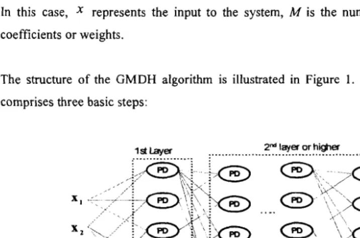
In this case, x represents the input to the system, M is the number of inputs and a are coefficients or weights.

The structure of the GMDH algorithm is illustrated in Figure 1. The computation process

comprises three basic steps:

Input \Ariables

Figure 1: Basic Structure ofGMDH

t value obtained I

Step 1: First n observations of regression-type data are taken. These observations are divided into two sets: the training set and testing set. The first layer model is obtained in every

column of the training sample of observations. The candidate models for first layer have the realization of the n

form:

'performances of tl

ated and is selectee

To obtain the value of the coefficients a for each rn models, a system of Gauss normal equations is solved. The coefficient Q; of nodes in each layer are expressed in the form

A. I

=

(X:X. I I)-1 X: Z I

where

number of observations in the training set.

Step 2: Construct

M'

=

M(M

-1) / 2 new variables in the training data set for all

possibilities of connection by each pair of neurons in the layer. A small number of variables

that give the best results in the first layer, are allowed to form second layer candidate models

of the same form:

Step 3: Select the single best neuron out of these

M'

neurons,

x',

according to the value of

mean square error (MSE). The MSE is defined by the formula:

1

n

MSE

=-

L(Y; -

Z;)2

nV;=nlr+1

where nv is the number of observations in the testing set, n is the total number of observation,

Z is the estimated output value and s is the model whose fitness is evaluated. Once the single best neuron,

x'

is selected, the MSE in each layer is further checked to determine whether the

set of equations of the model should be further improved within the subsequent computation.

MAE

=

RMSE

e Y1 and

z,

are th

EMPIRICAL RES

location in 1995 is

The lowest value of the selection criterion obtained during this iteration is compared with the smal1est value obtained at the previous one. If an improvement is achieved, then set new input :d

ry

{XI'

x z"'" x

m

_,x'},

_{M' =M'}

_{+1 and repeat steps 2 and 3. Otherwise the iterations terminate}

ie and a realization of the network has been completed.

The performances of the each model for both the training data and forecasting data are evaluated and is selected according to the mean absolute error (MAE) and root-mean-square error (RMSE), which are widely used for evaluating results of time series forecasting. The MAE and RMSE are defined as

MAE=~

il

Y1

_-ZII

N

I~I

Y

1

e

1 N z

RMSE

= -

I(y,

-zJ

N I=!

where Y, and

z,

are the observed and the forecasted rice yields at the time t. The criterions to judge for the best model are relatively smal1 of MAE and RMSE in the modeling and forecasting.

4. EMPIRICAL RESULTS

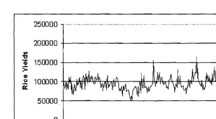
In our study, the data were collected from Muda Agricultural Development Authority (MUDA) Kedah, Malaysia ranging from 1995 to 2001 is used to validate the GMDHM algorithm for rice yields modeling. The results are compared with those the ANN. These time series come from different location and have different statistical characteristics. The rice yields data contains the yields data from 1995 to 200 I, giving a total of 351 observations. Given a set of 35 I observations made at uniformly spaced time intervals, the locations of rice

yield are rescaled to the time axis becomes the set of integers {I, 2, ..., 432} . For example the

first location in 1995 is written as time I, the second location in 1995 as time 2 and so on. The time series plot is given in Figure 2.

I -250000

200000 Based on these

."

"

4i 150000

e as inputs for the p

>=

<II

Q

ii

_{mplex, non-linear an}

50000 _{ochs using the back­}

0 efficient of 0.9. Tabl

51 101 151 201 251 301

Time

Figure 2. Rice Yields Series (1995-2001)

To assess the forecasting performance of different models, each data set is divided into two

samples. The first series was used for training the network (modeling the time series) and the

remaining were used for testing the performance of the trained network (forecasting). We take

the data from 1995 to 2001 producing 351 observations for training purpose and the

remainder as the output sample data set with 27 observations for forecasting purpose.

5 FITTING NEURAL NETWORK MODELS TO THE DATA

In this investigation, we only consider the situation of one-step-ahead forecasting with 27

observations. Before the training process begins, data normalization is often performed. The

linear transformation formula to [0, I] is used

x

_•

=A

Ymax

where

x.

and

Yo

represent the normalized and original data; and

Ymax

represent the

maximum values among the original data. In order to conform the neural network used in the

forecast, autocorrelation function (ACF) and partial autocorrelation function (PACF) were

used to determine the maximum number of input neurons used during the training (Cadenas

---_.­

4

4

I

neurons in the

3 9

1573

16093 3

0.118 O.l2S

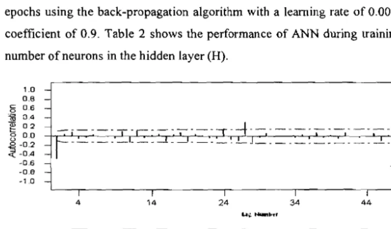
& Rivera, 2007). Figure 3 presents the ACF and PACF of data sets for the rice yields time series.

Based on these analyses, the maximum number of lags, 27, was identified suitable to

use as inputs for the proposed ANN. The one only neuron in the output layer represented

being modeled. All the data were normalized in the range

a

and I. After the input and out

variables were selected, the ANN architecture of 27-H-l was explored for capturing the

complex, non-linear and seasonality of rice yields data. The network was trained for 5000

epochs using the back-propagation algorithm with a learning rate of 0.00 I and a momentum coefficient of 0.9. Table 2 shows the performance of ANN during training with varying the

•

5

number of neurons in the hidden layer (H).

1.0 ­ 0.8 ­

g

0,6 ­

., 0.4 ­

~ 02 -

---r---,--f---,...-T---­

8 0.0

~:~~

::: I-- -- -

_ I . - - - J - - - . - - - ­

-0.6 ­ -0.8 ­

-'.0 ­

L---,---,---.---,---.---,---,-J_{I I} o

4 14 24 34 44 54

e

~

~:~

­ ~

'"

0.6

o 0.4 ­

u 0.2

---·----~1---·

~ 0.0

::: It·

- - . -t- -

r- -

-

~

-

. . . ­

-I· <J: -0.2

1ij -0.4

~ -0.6 ­

Q. -0.8 -1.0

I I I

I I

4 14 44 54 64

Figure 3: The ACF and PACF for the data study

Table 2 Performance Variation of a Three-Layer ANN during training with the number of

neurons in the hidden layer for ANN

Criterion Number of neurons in the hidden layer

3 9 15 21 27 33 39 45 51 57 63 70

1573 1504 1376 1319 1279

RMSE 16093 3 3 14263 14197 13794 8 12863 9 13334 12590 I MAE 0.118 0.1290.1150.114 0.114 0.113 0.1060.099 0.1020.103 0.097 0.101

It is observed that the performance of ANN is improved as the number of hidden neurons increases. However, too many neurons in the hidden layer may cause over-fitting problem, which results in the network can learn and memorize the data very well, but lacks the ability to generalize. If the number of neurons in hidden layer is not enough then the network may not be able to learn. So, an ANN with 63 neurons in the hidden layer seems to be appropriate.

6 FITTING GMDH MODELS TO THE DATA

In designing the GMDH model, one must determine the following variables: the number of input nodes, the number of hidden layers and the number of output. The selection of the number of input corresponds to the number of variables play important roles for many successful applications of GMDH. The issue of determining the optimal number of input nodes is a crucial yet complicated one. There is no theory that can used to guide the selection the number of input.

In this study, the ACF and PACF are used also to select the number of input nodes. Based on these analyses, the maximum number of lags, 27, was identified suitable to use as inputs for

the proposed GMDHM. The input pattern was assigned as x(t -1), x(t - 2), ... ,x(t -

27)

and thus the output pattern is:

yet) = f(x(t -l),x(t - 2), ...,x(t -

27))

The values predicted by the GMDH were compared with the ANN model. Table I shows the comparison of modeling/forecasting precision among the two approaches based on two statistical measures. In Table 1, the lowest RMSE and MAE are found with the ANN in the modeling while the GMDH in forecasting. The result, demonstrating that the GMDH provides a better approach for forecasting rice yields data.

Table 1 Comparison of modeling and forecasting precision among the four algorithms

Algorithms ANN GMDHZ

Modelling RMSE 12540.19 13431.18

MAE 0.0989 0.1038

Forecasting RMSE 16245.206 7549.243

MAE 0.1071 0.0512

CONCLUSI

Chang, F. J. aru forecast,

Hydro

Coulibaly, P., j

Networks modi 37(4),885-896

Hsu, K.L., GUf modelling ofra

Imrie, C.E., D, Networksuru: C

138-153.

7

CONCLUSION

This study investigated the applicability and capability of the GMDH model in rice yields forecasting. The performances of the GMDH model and observations were compared and evaluated based on their performance in the training and testing sets. The ANN models was also investigated for the same set of data and the results are reported. Based on the performance of two models, it can be concluded that GMDH is an effective method to forecast rice yields while the ANN method is superior to the GMDH method in the modeling of time-series. The results show that the combine the ANN and GMDH can be applied successfully to establish time-series forecasting models, which could provide accurate forecasting and modeling of time-series.

ACKNOWLEDGEMENTS

Special thanks to Ministry of Science, Technology and Innovation (MOSTI) for funding this research and MADA for their contribution of data.

REFERENCES

[1] Chang, F. 1. and Hwang, Y.Y. A self-organization algorithm for real-time flood forecast, Hydrological processes. 13,123-138.

[2] Coulibaly, P., Anctil, F., Aravena, R. and Bobee, 8., (2001), Artificial Neural Networks modelling of water table depth fluctuations, Water Resources Research, 37(4),885-896.

[3] Hsu, K.L., Gupta, H.V. and Sorooshian, S., (1995), Artificial Neural Networks modelling of rainfall-runoff process, Water Resources Research, 31(10), 2517- 2530.

[4] Imrie, C.E., Dean, S. and Korre, A., (2000), River flow using Artificial Neural Networksuru: Generalization beyond the calibration range, Journal ofHydrology,233 ,

138-153.

[5] Islam, S. and Kothart, R, (2000), Artificial Neural Networks in Remote Sensing of Hydrologic Processes, Journal ofHydrologic Engineering, 5(2), 138-144.

[6] Ivakheneko A G. and Ivakheneko, G.A. (1995), The review of problems solvable by algorithms of the GMDH, Pattern Recognition and Image Analysis, 5(4): 527­

[7] Khush, G.S., "Harnessing Science and Technology For Sustainable Rice Based Production Systems", Conf. on Food and Agricultural Organization Rice Conference, 2004.

[8] Madala, H.R. and Ivakhnenko, A.G. (1974). Inductive Learning Algorithmsfor Complex System Modeling. Boca Raton: CRC.

[9] Maier, H.R. and Dandy, G.C., (2000), Neural Networks for the production and forecasting of water resource Environmental modelling and software variables: a review and modelling issues and application, , 15, 101-124.

[10] Mark S. Voss and James C. Howland Ill. (2003). Financial Modelling using Social Programming. FEA 2003: Financial Engineering and Applications

[11] Mohammadi K, Eslami HR, Kahawita R. 2006. Parameter estimation of an ARMA model for river flow forecasting using goal programming. Journal of Hydrology 331: 293-299.

[12] Moradkhani, H, Hsu, K.L. Gupta, H.V. and Sorooshian, S, (2004). Improved streamflow forecasting using self-organizing radial basis function Artificial Neural Networks, Journal ofHydrology, 295, 246-262.

[13] Tamura, H. and Kondo, T. (1980). Heuristics Free Group Method of Data Handling Algorithm of Generating Optimal Partial Polynomials with Application to Air Pollution Prediction. Int. J System Sci. 1I: I095- 11I I.

[14] Tamura, H., and Kondo, T. (1980), Heuristics free group method of data handling algorithm of generating optimal partial polynomials with application to air pollution prediction, Int. J Syst. Sci., 11, 1095-1 I I 1.

[15] Thirumalaiah, K. and Deo, M.C., (2000), Hydrological Forecasting Using Neural Networks, Journal of Hydrologic Engineering, 5(2), 181-189.

[16J Tokar, A.S. and Markus, M., (2000), Precipitation-Runoff Modelling Using Artificial Neural Networks and Conceptual Models, Journal ofHydrologic Engineering, 5(2),

156-161.

[17] Tong, X.H., Kuang, J.C., Wang X.Y. and Qi, TX., (1996), Setting up prediction

model of gas well prediction rate by various methods. Natural Gas Industry, 16(6),

49-53.

[18] Wu Jr. S., Han J, Annarnbhotla S. and Bryant, S., (2005), Artificial Neural Networks

for Forecasting Watershed Runoff and Stream Flows, Journal ofHydrologic

Engineering, 5(2), 216-222.

[19] Yim, J. and Mitchell,H. Comparison of country risk models: hybrid neural networks,

logit models, discriminant analysis and cluster techniques, Expert Systems with

Applications 28 (2005) (1), pp. 137-148.

[20] Zealand, C.M., Bum, D.H. and Simonovic, S.P., (1999), Short term stream flow

forecasting using Artificial Neural Networks, Journal ofHydrology, 214, 32-48.

[21] Zhang, G.P. (2003). Time Series Forecasting Using a Hybrid ARIMA and Neural

Network Model. Neurocomputing 50: 159-175.

[22] Zou, H.F., Xia, G.P., Yang, F.T. & Wang, H.Y. (2007). An Investigation and Comparison of Artificial Neural Network and Time Series Models for Chinese Food

Grain Price Forecasting. Neurocomputing, 70: 2913-2923.