An Extension of RSS-based Model Comparison Tests for Weighted
Least Squares
H.T. Banks, Zackary R. Kenz, and W. Clayton Thompson
Center for Research in Scientific Computation
Center for Quantitative Sciences in Biomedicine
North Carolina State University
Raleigh, NC 27695-8212
August 22, 2012
Abstract
We consider residual-sum-of-squares-based model comparison tests using weighted least squares formula-tions and asymptotic statistics. An biological example from cell proliferation investigaformula-tions is presented in some detail to illustrate usefulness of the new results.
AMS subject classifications: 34A55, 62F03, 62F12, 93E24.
1
Introduction
Model comparison by hypothesis testing is a tool in inverse or parameter estimation problems to distinguish mathematically relevant features in a biological or physical system under study. Consider that one has some dynamical system which describes a biological process
dy
dx =g(x, y(x;q), q) (1)
y(0) =y0.
Given a set of observations of some component(s) of the system under study at various instances in time, it is a standard inverse problem to determine the value of the model parameterq, out of a setQof admissible parameters, which best describes the observed data. But an equally important problem is to establish, on a quantitative basis, that the biophysical mechanisms represented in the mathematical model are necessary to describe the observed data, and that no extraneous mechanisms have been included. This is the role of model comparison tests.
For certain classes of models, potentially extraneous mechanisms can be eliminated from the model by a simple restriction on the underlying parameter space, while the form of the mathematical model (1) remains unchanged. For instance, consider the convection-diffusion model
∂u ∂t +V
∂u ∂x =D
∂2u
∂x2,
where D is the diffusion coefficient and V is the bulk velocity of a transporting fluid. Such a model has been used to describe the transport of labeled sucrose in the brain tissue of cats [4]. Yet if the cerebral transport of sucrose is primarily driven by diffusion, then the convection term in the model above is extraneous. Given data involving the transport of labeled sucrose, one would like to compare the accuracy of two mathematical models. In the first, both convection and diffusion play a role and one must estimate the parameters V and D in an inverse problem. In the second, it is assumed that convection is not present (V = 0), and only the coefficient of diffusionDis estimated. Thus, in effect one has two mathematical models which must be compared in terms of how accurately and parsimoniously they describe an available data set. Equivalently, this problem can be cast in the form of a hypothesis test: one would like to test the null hypothesisV = 0, against the alternative hypothesis thatV 6= 0. Under the null hypothesis, the restricted mathematical model is contained within the mathematical model subject to the unconstrained parameter space (in the sense that estimating bothV andDsimultaneously includes the possibility thatV = 0). For this reason, the unconstrained model must necessarily fit the data (in an appropriate sense) at least as accurately as the constrained model. The role of the hypothesis test is to compare these two models on a quantitative basis to investigate whether the model withV 6= 0 provides a significantly (in some sense) better fit to the data.
As the above example makes clear, there is some similarity between model comparison testing and hypothesis testing for a set of mathematical models which have the same mathematical form but differ in the restrictions placed on the underlying parameter space. In such a case, one may resort to hypothesis testing as a technique for model comparison. In this note, we are interested in the situation where the parameter set for the restricted model,QH, can be identified as a linear subset of the admissible parameter set of the unrestricted model,Q(this
notation will be defined explicitly in Section 3). In addition to the study of convective mechanisms in models of fluid transport in cat brains [4], hypothesis tests have also been used to investigate mortality and anemotaxis in models of insect dispersal [5, 6]. These examples are summarized (focusing on the role of hypothesis testing) in [2, 8]. More recently, model comparison by hypothesis testing has been conducted to investigate the division dependence of death rates in a model of a dividing cell population [10], to evaluate the necessity of components in viscoelastic stenosis models [26], and to serve as the basis for developing a methodology to determine if a stenosis is present in a vessel based on input amplitude [3]. Thus the discussions and methods presented here have widespread applications in biological modeling as well as in more general scientific modeling efforts.
likelihood of a set of observations. Alternatively, one can use information theoretic model comparison tests such as Akaike’s Information Criterion (AIC) or similar tests (BIC, TIC, etc.) [14]. Still, such tests typically require a complete likelihood specification. Though a least squares analog of the AIC test exists, it is only valid if all observations are considered to be sampled from identical normal distributions with a constant variance (i.e.,i.i.d.
normal).
Unlike likelihood estimation, least squares estimation generally requires only the first two statistical moments of the observations to be specified [13, Ch. 3]. Additionally, the mathematical formulation is intuitive, and the resulting estimates are more robust to error misspecification (when compared to likelihood estimation) [17, Ch. 2]. As such, there is an obvious appeal for model comparison tests which are easy to apply in a least squares framework. Given the above discussion regarding the relationship between model comparison and hypothesis testing for certain classes of problems, we focus our attention on model comparison in a least squares framework. Hypothesis testing for least squares problems was considered at length by Gallant [19]. Subsequently, these results were reconsidered by Banks and Fitzpatrick [2] under a slightly different set of assumptions to develop a hypothesis test which could be computed from the residual sum of squares (RSS) after fitting the models to a data set in a least squares framework. Unfortunately, this work was limited to cases in which the observations were assumed to be characterized by constant variance. Both the works of Gallant as well as Banks and Fitzpatrick rely upon an asymptotic theory for nonlinear least squares to demonstrate their results.
In this presentation we begin by defining a general least squares estimation problem. Next, we review features of the asymptotic theory relevant to model comparison by hypothesis testing. Finally, we further extend the results of Banks and Fitzpatrick (in a manner suggested possible by Gallant) to a more general variance model. An example involving cell proliferation models with nonconstant variance in the experimental data is used to illustrate application of the new model comparison techniques.
2
Least Squares Estimation
We begin with the dynamical system (1) above, which describes some hypothesized mathematical relationship between an observed processy∈Rk, an independent variable (covariate)x∈Rm, and a set of parametersq∈Q. For notational convenience, we assume without loss of generality that k= 1. Letf(x;q) be the solution to (or observation for) the dynamical system. Suppose also that observations of the underlying process are noisy (that is, subject to random error and/or fluctuations). Following standard inverse problem procedures [13, 15, 17, 24], we may relate the mathematical model to the noisy data via a statistical model,
Yk =f(xk;q∗) +Ek. (2)
Here,{Ek}nk=1are random variables which account for any error (measurement error, modeling error,
microfluctu-ations, etc.) between the mathematical model and the recorded observations at values{xk}nk=1of the independent
variable. Hence the{Yk}nk=1are also random variables. It is assumed here that the values{xk}are known exactly.
The parameter q∗ is the hypothetical ‘true’ parameter which is assumed to generate the data for the observed process. It has been tacitly assumed that the underlying biological or physical system is perfectly represented by the mathematical model. (In fact, any mathematical model is only an approximation to reality. For the sake of argument, one can assume that the mathematical model is sufficiently accurate so that any modeling error is sub-sumed within the error random variablesEk. One can relax this assumption, though doing so greatly complicates
[18, 19] the analysis presented below.) It is further assumed that the error random variables are independent, though not necessarily identically distributed, with central moments
E[Ek] = 0, 1≤k≤n,
V ar(Ek) =σ2w(xk)2, 1≤k≤n.
With the assumptions and definitions above, we may define theweighted least squares cost function,
JnW LS(q) =
1 n
n
X
k=1
Yk−f(xk;q)
w(xk)
2
Theweighted least squares estimator is defined to be the random variableqW LS
n which minimizes the weighted
least squares cost function for a given set of random variables{Yk}, that is,
qnW LS = arg min q∈Qad
JnW LS(q), (4)
whereQad⊂Qis the set of admissible values for the parameterq. We remark that qnW LS is a random variable
which is dependent upon the random variables{Yk}(and hence the error random variables{Ek}). This dependence
is suppressed in the notation above (with the exception of the subscript n) for simplicity and clarity, although we can writeqW LS
n =qW LSn ({Yk}) when necessary. In the eventw(xk) = 1 for all 1≤k≤n, the formulas above
reduce down to the familiar ordinary least squares formulae
JnOLS(q) =
1 n
n
X
k=1
(Yk−f(xk;q))2, (5)
qnOLS= arg min q∈Qad
JnOLS(q). (6)
Finally, we remark that it is often convenient to use a vectorized notation for the least squares problems. Define ~
f(q) = (f(x1;q), . . . , f(xn;q))T. Then the statistical model (2) may be rewritten as
~
Y =f~(q) +E~ (7)
where
E[E~] =~0
Cov(E~) =σ2diag(w(x1)2, . . . , w(xn)2)
=σ2W.
Then clearly we can rewrite
JnW LS(q) =
1 n
~
Y −f~(q)TW−1Y~
−f~(q) (8)
JnOLS(q) =
1 n
~
Y −f~(q)TY~ −f~(q). (9)
The goal of an inverse or parameter estimation problem is to use a set of observations{yk}(realizations of the
random variables{Yk}) in order to determine an estimate of the true underlying parameterq∗. Intuitively, since
E[Yk] =f(xk;q∗) for all 1≤k ≤n, we would expect the least squares estimator (either qW LSn or qOLSn ) to be
‘close’ toq∗ in an appropriate sense. In practice, one uses the realized data
{yk}to determine an estimate ˆqnW LS
or ˆqOLS
n which is a realization of the appropriate least squares estimator. In this paper, we are less interested in
the computational issues associated with finding an estimate and more interested in characterizing the statistical properties of the estimator itself. Since the estimator is a random variable, it is described not by a numerical value but rather by a probability distribution, and we may use results from asymptotic theory to characterize the distribution of the estimator.
Going forward, for notational simplicity the dependence of the estimators and cost functions on n may be suppressed (e.g., usingJOLS(q) instead of JOLS
n (q)). This is the case particularly during the discussions of the
cell proliferation example in Section 5.
3
Asymptotic Theory and Model Comparison for Ordinary Least
Squares
of Banks and Fitzpatrick [2]. As mentioned previously, the work of Banks and Fitzpatrick was partially inspired by the work of Gallant [19], and many of their results and assumptions are similar. In the discussion that follows, we comment on any differences between the two approaches that we feel are noteworthy. While Gallant’s work is remarkably general, allowing for a misspecified model and a general estimation procedure (both least mean distance estimators and method of moments estimators are included), we do not consider such generalities here. The comments below are limited to least squares estimation with a correctly specified model (recall the discussion following Equation (2) above).
In this section we follow [2] in focusing exclusively on asymptotic properties and model comparison for
i.i.d. (absolute) error models. The theoretical results of Gallant similarly focus on i.i.d. errors, though some
mathematical tools are discussed which help to address more general error models [19, Ch. 2; pgs. 156–157]. In fact, these tools are used in a rigorous fashion in the next Section to extend the results of [2].
We begin by establishing some notation and precisely defining the hypothesis testing problem. It is assumed that the error random variables are defined on some probability triple (Ω,F, P) and take their values in a spaceE. By construction, it follows that the data{Yk}as well as the estimatorsqW LSn andqnOLSare also random variables
defined on this probability triple, and hence are functions ofω ∈Ω so that we may write Yk(ω),qOLSn (ω), etc.,
as necessary.
As in the discussion of Section 2, we consider parametersq∈Qad⊂Qfor a topological spaceQ. Given the
model f(x;q) defined above, it is assumed that the sampled values of the independent variables satisfyxk ∈X
for allk, and for some metric spaceX. Moreover, if the setX is totally ordered (see Assumption (A3) below), then one can define the empirical distribution function,
µn(x) = 1
n
n
X
k=1
∆xk(x)
where
∆xk(x) =
0, x≤xk
1, otherwise .
Clearly,µn∈ P(X), the space of probability measures onX.
Finally, we return to the original goal of model comparison by hypothesis testing. For now, we use the notation of ordinary least squares estimation, in keeping with the results presented in [2]. We have already defined above the standard ordinary least squares estimator
qOLSn = arg min q∈Qad
JnOLS(q).
As alluded to in the introduction, we might also consider a restricted version of the mathematical model in which the unknown true parameter is assumed to lie in a subsetQH⊂Qad⊂Qof the admissible parameter space. We
assume this restriction can be written as a linear constraint,Hq∗
=h, whereH is a known linear function andh is a known vector. Thus the restricted parameter space is
QH ={q∈Qad:Hq=h}.
Then the null and alternative hypotheses are
H0:q∗∈QH
HA:q∗6∈QH.
We may define the restricted estimator
qOLS
n,H = arg min q∈QH
JOLS
n (q), (10)
and the corresponding estimate ˆqOLS
n,H. It is clear that JnOLS(ˆqnOLS)≤JnOLS(ˆqn,HOLS), since QH ⊂Qad. This fact
With these definitions, attention can now be directed toward establishing a quantitative basis upon which the null hypothesisH0should either be accepted or rejected. Again, the results presented below are paraphrased
from [2], and comments have been included to indicate the alternative approach due to [19]. No proofs are given here, though the interested reader can find a complete set of proofs in [2] and [19]. First, we consider the following set of assumptions:
(A1) The error random variables{Ek} are independent and identically distributed random variables with
distri-bution functionP(E). Moreover,E[E~] =~0 andCov(E~) =σ2I
n whereIn is then×nidentity matrix.
(A2) Qis a separable, finite-dimensional topological space (i.e., Q⊂Rp), andQad is a compact subspace ofQ
withq∗
∈int(Qad).
(A3) X is a compact subset ofRm.
(A4) The functionf(·;·)∈C2(Q, C(X)).
(A5) There exists a finite measure µonX such that
1 n
n
X
k=1
g(xk) =
Z
X
g(x)dµn(x)→
Z
X
g(x)dµ(x)
for all continuous functionsg. That is, the probability distributionsµnconverge weakly toµ, orµnconverges
toµin the weak∗topology (whenP(X) is viewed as a subset ofC∗(X), the dual of the space of continuous functions).
(A6) The functional
J∗
(q) =σ2+
Z
X
(f(x;q∗
)−f(x;q))2dµ(x) has a unique minimizer atq∗
∈Qad.
(A7) The matrix
J = ∂
2J∗(q∗) ∂q2
= 2
Z
X
∂f(x;q∗) ∂q
∂f(x;q∗)T
∂q +
∂2f(x;q∗) ∂q2 (f(x;q
∗
)−f(x;q∗ ))
dµ(x)
= 2
Z
X
∂f(x;q∗) ∂q
∂f(x;q∗)T
∂q
dµ(x)
is positive definite.
(A8) The matrix H, of dimensionr×p, has full rankr.
The most notable difference between the assumptions above (which are those of [2]) and those of [19] is assumption (A5). In its place, Gallant states the following.
(A5′) Define the probability measure
ν(S) =
Z
X
Z
E
IS(E, x)dP(E)dµ(x)
for a set S ⊂ E×X and µ defined as above. Then almost every realized pair (ǫk, xk) is a Cesaro sum
generator with respect toν and a dominating functionb(E, x) satisfyingR
X×Ebdν <∞. That is,
lim
n→∞ 1 n
n
X
k=1
g(ǫk, xk) =
Z
X
Z
E
almost always, for all continuous functionsg such that|g(E, x)|< b(E, x). Moreover, it is assumed that for eachx∈X, there exists a neighborhoodNx such that
Z
E
sup
Nx
b(E, x)dP(E)<∞.
The assumption (A5′
) is stronger than the assumption (A5) as it supposes not only the existence of a dominating function, but also involves the behavior of the probability distributionP, which is generally unknown in practice. The practical importance of the dominating function b arises in the proof of consistency for the least squares estimator (see Theorem 3.1 below). As has been noted elsewhere (see, e.g., [1], [24, Ch. 12]), the strong consistency of the estimator is proved by arguing thatJ∗(q) is the almost sure limit of JOLS
n (q). Thus,
ifJOLS
n (q) is ‘close’ to J∗(q) andJ∗(q) is uniquely minimized byq∗, it makes intuitive sense that qOLSn , which
minimizes JOLS
n (q), should be close to q∗. This task is made difficult by the fact that the null set (from the
‘almost sure’ statement) may depend on the parameterq. In [2], the almost sure convergence ofJOLS
n (q) toJ∗(q)
is demonstrated constructively; that is, by building a set A∈ F (which does not depend on q) withP(A) = 1 such thatJOLS
n (q)→ J∗(q) for eachω ∈A and for eachq ∈Q. This construction relies upon the separability
of the parameter spaceQ(assumption (A2)) as well as the compactness of the spaceX (assumption (A3)). The alternative approach of Gallant uses a consequence of the Glivenko-Cantelli theorem [19, pg. 158] to demonstrate a uniform (with respect to q) strong law of large numbers. The proof relies upon the dominated convergence theorem, and hence the dominating function b. As a result, Gallant does not need the space Qto be separable or the spaceX to be compact. It should be noted, however, that in most practical applications of interestQand X are compact subsets of Euclidean space so that relaxing these assumptions provides little advantage.
The choice of dominating function b(E, x) deserves further comment. Define the functional h:E×X →R
by
h(E, x) = (E+f(x, q∗
)−f(x, q))2. Then b(E, x) is chosen so that h, as well as its derivatives ∂q∂h
i,
∂2h
∂qi∂qj and the product terms ∂h ∂qi
∂h
∂qj (for all
combinations of 1≤i, j≤p), are dominated bybfor allq∈Q[19, pg. 256]. The domination of the functionhby theν-integrable functionbcan be used to obtain a number of desirable results, including uniform convergence and the interchange of differentiation and integration [19, Lemma 3]. As a result, one does not need a positive definite hessian matrixJ to prove the asymptotic normality of scores [19, Thm. 4] (contra. [2, Thm. 4.1]). Rather, one only needsJ to be nonsingular in order for the conclusion of Theorem 3.2 below to be well-defined.
While the list of assumptions above is extensive, we remark that the set is not overly restrictive. Assumptions (A2) and (A3) are naturally satisfied for most problem formulations (although the requirementq∗
∈int(Qad) may
be occasionally problematic [2, Remark 4.4]). Assumptions (A4) and (A8) are easily checked. Though assumption (A1) may be difficult to verify, it is much less restrictive than, say, a complete likelihood specification. Moreover, residual plots [13, Ch. 3] can aid in assessing the reliability of the assumption.
Assumption (A5) is more difficult to check in practice as one does not know the limiting distribution µ. Of course, this is simply an assumption regarding the manner in which data is sampled (in the independent variable space X)–namely, that it must be taken in a way that ‘fills up the space’ in an appropriate sense. Similarly, assumptions (A6) and (A7) cannot be verified directly as one knows neither µ nor q∗. In many practical applications of interest,µis Lebesgue measure, and one can assess the assumptions atqOLS
n (which is
hopefully close toq∗
). Of course, if assumption (A7) holds, then assumption (A6) must hold at least for a small region aroundq∗
, though possibly not on all ofQad.
As noted above, assumption (A7) is not strictly necessary if one uses assumption (A5′
) in the place of (A5). Given assumptions (A2)–(A4), it follows that the functionh(and its relevant derivatives; see above) is bounded (and hence dominated by aν-measurable function) provided thespaceE in which the random variables Ek take
their values is bounded. On one hand, this has the desirable effect of weakening the assumptions placed on the Hessian matrixJ. Yet the assumption thatE is boundedprecludes certain error models, in particularnormally
distributed errors.
in the restricted parameter space
˜ QH=
n
q∈Qad: ˜H(q) = ˜h
o
.
Assuming the null hypothesis is true, one can construct the linearization
L(q) = ˜H(q∗
) +∂H˜(q ∗) ∂q (q−q
∗ )
= ˜h+∂H˜(q ∗) ∂q (q−q
∗ ).
Then
˜ QH≈
n
q∈Qad:L(q) = ˜h
o
.
But the conditionL(q) = ˜his equivalent to the condition that
∂H˜(q∗) ∂q q=
∂H˜(q∗) ∂q q
∗ .
Thus, under the null hypothesis, the nonlinear restriction ˜H(q∗
) = ˜his asymptotically locally equivalent to the linear restriction of assumption (A8) withH = ∂H˜∂q(q∗) andh= ∂H˜∂q(q∗)q∗. As such, we only consider the problem of testing a linear hypothesis. For nonlinear hypotheses, the results presented here are accurate to the order of the linear approximations above.
We now give several results which summarize the asymptotic properties of the ordinary least squares estimator.
Theorem 3.1. Given assumptions (A1)–(A6),qOLS
n →q
∗
with probability one. That is,
Pnω∈Ω q
OLS
n (ω)→q
∗o = 1.
This theorem states that the ordinary least squares estimator is consistent. We remark that the finite dimen-sionality of the parameter spaceQ(see assumption (A2)) is not necessary in the proof of this theorem, and it is sufficient for the functionf to be continuous fromQinto C(X) rather than having two continuous derivatives.
Given Theorem 3.1, the following theorems may also be proven.
Theorem 3.2. Given assumptions (A1)–(A7), asn→ ∞
√
n qnOLS−q
∗ D
−→ N 0,2σ2J−1
,
where the convergence is in distribution, and occurs with probability one.
Theorem 3.3. Given assumptions (A1)–(A8) and assuming H0 is true, then as n→ ∞
√
n qn,HOLS−qOLSn
D
−→ N 0,J−1V
J−1
where
V = 2σ2HT(H
J−1HT)−1H.
Again, the convergence occurs with probability one.
In effect, Theorem 3.3 states that the restricted and unrestricted OLS estimators will converge to one another providedH0is true. Now we can turn to the main result of interest. Define
UnOLS =
n JOLS
n (qOLSn,H )−JnOLS(qnOLS)
JOLS n (qOLSn )
Theorem 3.4. Under assumptions (A1)–(A8) and assuming H0 is true, then as n→ ∞
UnOLS
D
−→χ2(r)
with probability one, whereχ2(r)is a Chi-square distributed with rdegrees of freedom.
Proofs of Theorems 3.1–3.4 can be found in [2]. We remark again that very similar results (under slightly differing assumptions) can be found in [19] where it is shown that the statistic
˜ UnOLS=
(n−p) JOLS
n (qOLSn,H )−JnOLS(qnOLS)
JOLS n (qnOLS)
is asymptotically distributed asχ2(r) [19, pg. 236]. The two model comparison statistics UOLS
n and ˜UnOLS are
asymptotically equivalent, the difference in scaling factors amounting to a bias correction in the estimation of the variance parameterσ2. See [2, Thm. 4.6] and [19, pg. 236] for details.
The practical importance of this theorem is that one has a quantitative basis upon which to assess the null hypothesis. Because the unrestricted model contains the restricted model as a special case, we must have JOLS
n (ˆqn,HOLS)≥JnOLS(ˆqnOLS) and thus ˆuOLSn ≥0 where ˆuOLSn is a realization ofUnOLS. Heuristically,UnOLS is used
to indicate the relative likelihood that the results obtained from a given realization of the data are the result of random chance. A full discussion of the use and interpretation of the test statistic is given in [2, pg. 518–519] and [13, Sec. 3.5.1]. Significantly, the termsJOLS
n (ˆqOLSn ) andJnOLS(ˆqn,HOLS) used to compute ˆuOLSn are a natural
byproduct of the optimizations (6) and (10) and can be returned directly by most optimization software. It should also be noted that the limiting distribution forUOLS
n is independent of the model parameterization. As such, the
results are robust to any reparameterization or change of variables in the mathematical modelf(x;q).
4
Extension to Weighted Least Squares
The results presented above are quite useful, but they only apply to the class of problems in which the error random variables are independent and identically distributed with constant varianceσ2. While the assumption
of independence is common, there are many practical cases of interest in which these random variables are not identically distributed. As discussed in Section 2, one may encounter a weighted least squares problem in which E[Ek] = 0 for allk butV ar(Ek) =σ2w(xk)2. In such a case, the results above (namely, assumption (A1)) fail to
apply directly. See, e.g., [7, Sec. 2] and references therein as well as [13] for more information on the development of error models.
In order to extend the results presented above to independent, heteroscedastic error models (and hence, to weighted least squares problems), we turn to a technique suggested by Gallant [19, pg. 124] in which one defines a change of variables in an attempt to normalize the heteroscedasticity of the random variables. As has been noted previously, Gallant used this technique under a different set of assumptions in order to obtain results similar to those presented above. This change of variables technique will allow us to extend the results above, originally from [2], in a rigorous fashion.
Consider the following assumptions.
(A1′a) The error random variables
{Ek} are independent and have central moments which satisfy E[E~] = ~0,
Cov(E~) =σ2W =σ2diag(w(x
1)2, . . . , w(xn)2).
(A1′b) The distributions of the random variables
{Ek}are completely determined by the first two central moments.
(A1′
c) The functionw:X →R+is continuous. (A7′
) The matrix
˜
J = 2
Z
X
1 w(x)2
∂f(x;q∗ ) ∂q
∂f(x;q∗ )T ∂q
dµ(x)
Theorem 4.1. Under assumptions (A1′a)–(A1′c), (A2)–(A6), (A7′), and (A8),
1. qW LS
n →q
∗
with probability one, and
2. √n qW LS
n −q∗
D
−→ N 0,2σ2 ˜
J−1.
Assuming further thatH0 is true,
3. √n qW LS
n,H −qW LSn
D
−→ N0,J˜−1V˜ ˜
J−1
where
˜
V = 2σ2HT(HJ˜−1HT)−1H.
Again, the convergence occurs with probability one. Finally, defining
UnW LS=
n JW LS
n (qn,HW LS)−JnW LS(qnW LS)
JW LS n (qW LSn )
,
4. UW LS
n
D
−→χ2(r)with probability one.
Proof. We first recall the statistical model (2)
Yk =f(xk;q∗) +Ek,
which can be written in vector form (7) as ~
Y =f~(q∗ ) +E~, where nowE[E~] =~0 andCov(E~) =σ2W. Define L=diag(w(x
1), . . . , w(xn)). It follows thatLLT =L2=W (L
is the Cholesky decomposition ofW). Also,L−1 exists and can be applied to both sides of (7) to obtain
L−1Y~ =L−1f~(q∗
) +L−1~
E
or ~ Z=~h(q∗
) +~η, (11)
whereZ~,~hand~η have the obvious definitions. The OLS cost functional for the transformed model and data (11) is
JnOLS(q) =
1 n
~
Z−~h(q)TZ~ −~h(q)
= 1 n
L−1Y~
−L−1f~(q)TL−1Y~
−L−1f~(q)
= 1 n
~
Y −f~(q)TL−1L−1Y~
−f~(q)
= 1 n
~
Y −f~(q)
T
W−1Y~ −f~(q).
In other words, the ordinary least squares cost function with respect to the transformed model and data (11) is exactly the weighted least squares cost function (8) for the original model and data. Thus, in order to prove Theorem 4.1, we will show that the rescaled model (11) satisfies the assumptions of Theorems 3.1–3.4.
Clearly,E[~η] =~0 andCov(~η) =σ2L−1W L−1=σ2I
n. Thus the random variablesηk (the components of~η)
that the functionh(x;q) =f(x;q)/w(x)∈C2(Q, C(X)). This follows from assumption (A1′c) and the fact that w(x) does not depend onq. For assumption (A6), we must show
˜ J∗
(q) =σ2+Z
X
(h(x;q∗
)−h(x;q))2dµ(x)
=σ2+
Z
X
f(x;q∗
)−f(x;q) w(x)
2
dµ(x)
has a unique minimum at q = q∗. Clearly, ˜J∗(q∗) = σ2. Since the function J∗(q) (see assumption (A6)) has a unique minimum at q = q∗ and w(x) >0, it follows immediately that ˜J∗(q∗) > σ2 ifq
6
= q∗ so that ˜J∗(q) has a unique minimum atq=q∗. Assumption (A7) is satisfied for the formulation (11) directly by assumption (A7′
).
In fact, the proof of Theorem 4.1 applies to any set of observations in which a change of variables can be used to produce a set of error random variables which are independent and identically distributed. The weighted least squares problem addressed in the above discussion arises from an observation process in which the errors are assumed to be independent but are not necessarily identically distributed. By rescaling the observations in accordance with their variance (which is assumed to be known) one obtains error random variables which are identically distributed as well as independent. Even more generally, it is not strictly necessary that the observations be independent. For instance, one might have observations generated by an autoregressive process of orderr. Then, by definition, some linear combination of r observational errors will give rise to errors which are independent and identically distributed. This linear combination is exactly the change of variables necessary to obtain a model which is suitable for ordinary least squares. Thus, even in the most general situation, when one hasCov(E~) =R, one may still use the Cholesky decomposition in the manner discussed above, provided one has sufficient assumptions regarding the underlying error process. See [19, Ch. 2] for details.
As in Section 3, the assumption (A7′) is the most problematic to verify in practice. In the proof above for the weighted least squares problem, the assumption (A1) has been replaced with assumptions (A1′a)–(A1′c), a change which merely accounts for the heteroscedastic statistical model. Then the assumptions (A2)–(A6) and (A8) for the rescaled model (11) can be verified directly from the original assumptions (A2)–(A6) and (A8) for the ordinary least squares formulation, as shown above. The only exception is the assumption (A7), which cannot be established directly from the ordinary least squares assumptions, hence the need for assumption (A7′
). On one hand, the existence of a unique minimum (assumption (A6)) is sufficient to prove that the matrix J or ˜J
must be positivesemi-definite, so that the assumption (A7) or (A7′
) may not be overly restrictive. Alternatively, as has been noted before, one can relax the assumptions (A7) or (A7′) by assuming the existence of a dominating function b. Moreover, provided the weightsw(x) satisfy the slightly stronger requirement w(x)≥δ > 0 for all x∈X, then one can use the dominating function b (from the ordinary least squares problem) to obtain a new dominating function ˜b(E, x) = δ−1b(
E, x) which is also ν-integrable. Even in this case, though, one must still make the additional assumption that ˜J is invertible.
All of the results above also readily extend to systems governed by partial differential equations; the essential elements of the theory are the form of the discrete observation operator for the dynamical system and the statistical model as given in (2).
5
Example: Hypothesis Testing in Models of Cell Proliferation
0 0.5 1 1.5 2 2.5 3 3.5 0
0.5 1 1.5 2 2.5 3 3.5x 10
5 Histogram Data, t =24 hrs
Log FI
Cell Counts
0 0.5 1 1.5 2 2.5 3 3.5
0 0.5 1 1.5 2 2.5 3 3.5x 10
5 Histogram Data, t =48 hrs
Log FI
Cell Counts
0 0.5 1 1.5 2 2.5 3 3.5
0 0.5 1 1.5 2 2.5 3 3.5x 10
5 Histogram Data, t =96 hrs
Log FI
Cell Counts
0 0.5 1 1.5 2 2.5 3 3.5
0 0.5 1 1.5 2 2.5 3 3.5x 10
5 Histogram Data, t =120 hrs
Log FI
Cell Counts
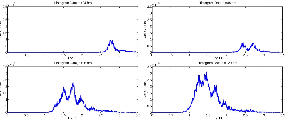
Figure 1: Typical histogram data for a CFSE-based proliferation assay showing cell count vs. log fluorescence intensity; originally from [22].
The mathematical modeling problem is to develop a system of equations which accounts for the manner in the population distribution of CFSE evolves as cells divide, die, and slowly lose fluorescence intensity as a result of protein turnover. In doing so, one must account for not only the division and death dynamics of the population of cells, but also how these processes relate to the observed distribution of fluorescence intensities. Let ˜ni(t,x˜)
represent the label-structured density (cells per unity of intensity, cells/UI) of cells at timet having completedi divisions and having fluorescence intensity ˜xfrom intracellular CFSE (that is, not including the contribution of cellular autofluorescence). Then it can be shown that this density can be modeled in terms of two independently functioning components, one accounting for the division dynamics of the population of cells, and one accounting for the intracellular processing of CFSE [20, 23]. It has been shown that the slow loss of fluorescence intensity as a result of intracellular protein turnover can be well-modeled by a Gompertz growth/decay process [9, 25]. It has also been shown that the highly flexible cyton model [21] can very accurately describe the evolving generation structure (cells per number of divisions undergone) [12]. Thus we consider the model
˜
n(t,x˜) =Ni(t)¯ni(t,x˜) (12)
The functions ¯ni(t,x˜) each satisfy the partial differential equation
∂¯ni(t,x˜)
∂t −ce
−kt∂[˜x¯ni(t,x˜)]
∂x˜ = 0 (13)
with initial condition
¯
ni(0,x˜) =
2iΦ(2ix˜)
N0
,
where Φ(x) is the label-structured density of the cells at t= 0, andN0 is the number of cells in the population
att= 0, all of which are assumed to be undivided. The functionsNi(t) are described by the cyton model,
N0(t) =N0−
Z t
0
ndiv0 (s)−ndie0 (s)
ds
Ni(t) =
Z t
0
2ndiv
i−1(s)−ndivi (s)−ndiei (s)
where ndiv
i (t) and ndiei (t) indicate the numbers per unit time of cells having undergone i divisions that divide
and die, respectively, at timet. In this regard, the cyton model (and hence, the mathematical model as a whole) can be considered as a large class of models differentiated by the mechanisms one uses to describe the terms ndiv
i (t) and ndiei (t), which we consider in more detail below. We remark that the mathematical model (12) can
be equivalently characterized by the system of partial differential equations ∂˜n0
∂t −ce
−kt∂x˜n˜0
∂x˜ = n
div
0 (t)−ndie0 (t)
¯ n0(t,x˜)
∂˜n1
∂t −ce
−kt∂x˜n˜1
∂x˜ = 2n
div
0 (t)−ndiv1 (t)−ndie1 (t)
¯ n1(t,˜x)
.. .
Given the solution ˜n(t,x˜) =P
˜
ni(t,x˜) in terms of the fluorescence resulting from intracellular CFSE, one must
add in the contribution of cellular autofluorescence to obtain a population density structured by total fluorescence intensity, which is the quantity measured by a flow cytometer. This density can be computed as
n(t, x) =
Z ∞
0
˜
n(t,x˜)p(x−x˜)dx,˜
wherep(xa) is a density function describing the distribution of cellular autofluorescence [20].
Letφ0(t) andψ0(t) be probability density functions (in units 1/hr) for the time to first division and time to
death, respectively, for an undivided cell. LetF0, the initial precursor fraction, be the fraction of undivided cells
which would hypothetically divide in the absence of any cell death. It follows that
ndiv0 (t) =F0N0
1−
Z t
0
ψ0(s)ds
φ0(t)
ndie0 (t) =N0
1−F0
Z t
0
φ0(s)ds
ψ0(t). (15)
Similarly, one can define probability density functionsφi(t) andψi(t) for times to division and death, respectively,
for cells having undergoneidivisions (he cellular ‘clock’ begins at the completion of the previous division), as well as the progressor fractionsFi of cells which would complete theith division in the absence of cell death. Then
ndivi (t) = 2Fi
Z t
0
ndivi−1(s)
1−
Z t−s
0
ψi(ξ)dξ
φi(t−s)ds
ndie i (t) = 2
Z t
0
ndiv i−1(s)
1−Fi
Z t−s
0
φi(ξ)dξ
ψi(t−s)ds. (16)
It is assumed that the probability density functions for times to division are lognormal, and that undivided cells and divided cells have two separate density functions. Similarly, it is assumed that divided cells die with a lognormal probability density. Thus
φ0(t) =
1 tσdiv
0
√
2πexp
−(logt−µ
div
0 )2
2(σdiv
0 )2
φi(t) =
1 tσdiv
i
√
2πexp
−(logt−µ
div i )2
2(σdiv i )2
(i≥1)
ψi(t) =
1 tσdie
i
√
2πexp
−(logt−µ
die i )2
2(σdie i )2
(i≥1).
We treat cell death for undivided cells as a special case. It is assumed that the density function describing cell death for undivided cells is
ψ0(t) =
F0
tσdie
0
√
2πexp
−(logt−µ
die
0 )2
2(σdie
0 )2
where pidle is the fraction of cells which are will neither die nor divide over the course of the experiment. The
form of the function above arises from the assumption that progressing cells die with a lognormal probability density. Nonprogressing cells die at an exponential rate, except for the fraction of idle cells. For the purposes of this paper, we are interested in testing the null hypothesispidle= 0 against the alternative hypothesispidle6= 0.
A more detailed discussion of the mathematical model can be found in [11].
With the mathematical model established, we now turn our attention to a statistical model of the data. Let Nkjbe a random variable representing the number of cells measured at timetjwith log-fluorescence intensity in the
region [zk, zk+1). Letqbe the vector of parameters of the model (12), so that we may rewriten(t, x) =n(t, x;q).
Define the operator
I[n](tj, zk;q) =
Z zk+1
zk
10zln(10)n(t,10z;q)dz,
which represents the computation of cell counts from the structured densityn(t, x) transformed to the logarithmic coordinatez= log10x. Then a statistical model linking the random variablesN
j
k to the mathematical model is
Nkj=λjI[ˆn](tj, zkj;q0) +λj
I[ˆn](tj, zkj;q0)
γ
Ekj (18)
where theλj are scaling factors [25, Ch. 4] and the random variablesEkj satisfy assumption (A1). In principle, it
is possible to use a multi-stage estimation procedure to determine the values of the statistical model parameters λj andγ [17] but we do not consider that here. It is assumed thatλj = 1 for allj.
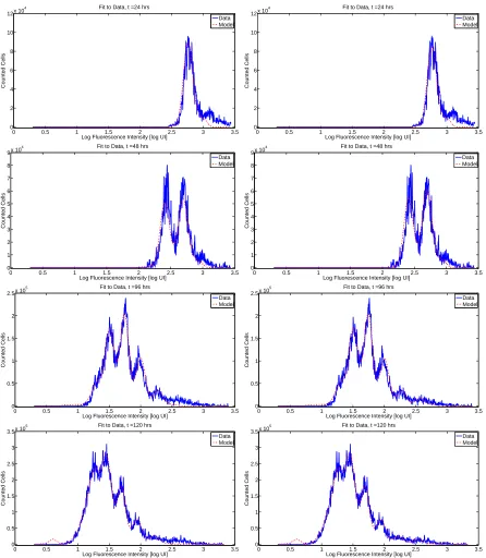
In the case thatγ= 0, one has precisely absolute error and a statistical model suitable for the ordinary least squares cost function (5) and estimator (6) to estimate the unknown parameterq0. The results of using the OLS
estimator can be found in Figure 2 for the null and alternative hypotheses. The ordinary least squares cost of fitting the model (12) under the null hypothesis isJOLS(ˆqOLS
H ) = 4.0423×10¹¹. The ordinary least squares cost
under the alternative hypothesis isJOLS(ˆqOLS) = 3.6228×10¹¹ [11]. We would like to determine whether or
not the small decrease in cost associated with the alternative hypothesis is outweighed by the larger number of parameters (17 versus 16) required. As seen in Figure 2, the fits of the two models to the data are very similar, so that one cannot justify a conclusion solely on the basis of the slightly reduced cost. Rather, one should use a model comparison test.
However, as the theory of Sections 3 and 4 suggests, one cannot rigorously apply a model comparison test unless the underlying statistical model is accurate. It follows from the form of Equation (18) that whenγ= 0 the residualsrjk=I[n](tj, zkj; ˆqOLS)−n
j
k (where then j
k are realizations of the data random variablesN j
k) correspond
to realizations of the error termsEkj. As such, these residuals should appear random when plotted as a function of the magnitude of the model solution [13, Ch. 3]. However, we see in Figure 3 (top) that this is not the case. There is a noticeable increase in the variance of the residuals as the magnitude of the model solution increases. Thus we must conclude that the constant variance modelγ= 0 is not correct, and that the ordinary least squares cost function is not adequate as a basis for model comparison. A constant coefficient of variation (CCV) model (γ= 1, usually calledrelative error) leading to a generalized least squares (GLS) problem formulation was also considered in [25]. Again residual analysis suggested that this was not the correct formulation.
In fact, the most appropriate theoretical value of γ appears to be γ = 1/2 [25] so that the weighted least squares cost function (3) and estimator (4) should be used. Because the weights must be bounded away from zero (see assumption (A1′
c)), we define the weights to be
w(tj, zkj) =
I[n](tj, zkj;q
∗)1/2, I[n](t
j, zkj;q
∗)> I∗ (I∗)1/2, I[n](t
j, zkj;q
∗)
≤I∗ .
The cutoff valueI∗
>0 is determined by the experimenter so that the resulting residuals appear random. In the work that follows,I∗= 1
×104. Becausewj
k depends upon the unknown parameterq
∗, an iterative optimization scheme must be used (see [13, Ch. 3] or [17, Ch. 2] for details). Using an estimate ofq∗ (say, the ordinary least squares estimate ˆqOLS), one computes the weights according to the formula above (with q∗ replaced by ˆqOLS)
and then uses these (fixed) weights to compute the weighted least squares estimate ˆqW LS. One can then use this
0 0.5 1 1.5 2 2.5 3 3.5 0 2 4 6 8 10 12x 10
4 Fit to Data, t =24 hrs
Log Fluorescence Intensity [log UI]
Counted Cells
Data Model
0 0.5 1 1.5 2 2.5 3 3.5
0 2 4 6 8 10 12x 10
4 Fit to Data, t =24 hrs
Log Fluorescence Intensity [log UI]
Counted Cells
Data Model
0 0.5 1 1.5 2 2.5 3 3.5
0 1 2 3 4 5 6 7 8 9x 10
4 Fit to Data, t =48 hrs
Log Fluorescence Intensity [log UI]
Counted Cells
Data Model
0 0.5 1 1.5 2 2.5 3 3.5
0 1 2 3 4 5 6 7 8 9x 10
4 Fit to Data, t =48 hrs
Log Fluorescence Intensity [log UI]
Counted Cells
Data Model
0 0.5 1 1.5 2 2.5 3 3.5
0 0.5 1 1.5 2 2.5x 10
5 Fit to Data, t =96 hrs
Log Fluorescence Intensity [log UI]
Counted Cells
Data Model
0 0.5 1 1.5 2 2.5 3 3.5
0 0.5 1 1.5 2 2.5x 10
5 Fit to Data, t =96 hrs
Log Fluorescence Intensity [log UI]
Counted Cells
Data Model
0 0.5 1 1.5 2 2.5 3 3.5
0 0.5 1 1.5 2 2.5 3 3.5x 10
5 Fit to Data, t =120 hrs
Log Fluorescence Intensity [log UI]
Counted Cells
Data Model
0 0.5 1 1.5 2 2.5 3 3.5
0 0.5 1 1.5 2 2.5 3 3.5x 10
5 Fit to Data, t =120 hrs
Log Fluorescence Intensity [log UI]
Counted Cells
Data Model
0 0.5 1 1.5 2 2.5 3 x 10⁵ −6
−4 −2 0 2 4 6x 10
4 Residual Plot
I[n](t
i,zk)
Residuals
0 0.5 1 1.5 2 2.5 3
x 105 −6
−4 −2 0 2 4 6x 10
4 Residual Plot
I[n](t
i,zk)
Residuals
0 0.5 1 1.5 2 2.5 3
x 105 −250
−200 −150 −100 −50 0 50 100 150 200 250
Modified Residual Plot
I[n](t
i,zk)
Modified Residuals
0 0.5 1 1.5 2 2.5 3
x 105 −250
−200 −150 −100 −50 0 50 100 150 200 250
Modified Residual Plot
I[n](t
i,zk)
Modified Residuals
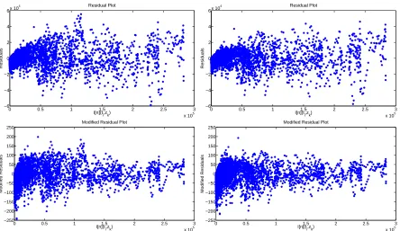
Figure 3: Top: residual plots for the mathematical model under the null (left) and alternative (right) hypotheses, showing the residuals in terms of the magnitude of the model solution. Bottom: modified residual plots for the mathematical model under the null (left) and alternative (right) hypotheses, showing the modified residuals in terms of the magnitude of the model solution. While the variance of the standard residuals is observed to grow with the magnitude of the model solution, we see that the variance of the modified residuals is largely constant.
Residual plots obtained using the theoretical value ofγ= 1/2 are shown in Figure 3 (bottom). (The weighted least squares fit to data is not shown, as the results are sufficiently similar to the ordinary least squares fits of Figure 2.) While the variance of the standard residuals is observed to increase with the magnitude of the model solution, the variance of the modified residuals is approximately constant, providing some evidence that the statistical model (18) (with γ = 1/2) is correct. As such, we are prepared to use the model comparison test statistic to analyze the null hypothesis.
Under the null hypothesis, the weighted least squares cost functional isJW LS(ˆqW LS
H ) = 10.3040×10⁶. Under
the alternative hypothesis, the weighted least squares cost functional is JW LS(ˆqW LS) = 8.8394×10⁶. Thus
the model comparison statistic is ˆuW LS ≈ 711.3 (there are 4293 data points). We conclude then, that there
is overwhelming evidence to reject the null hypothesis in favor of the alternative hypothesis. In the present
application, this strongly suggests that the fraction of cells which remain idle over the course of the experiment is a significant mathematical feature which should be included in an accurate model of proliferation assay data. As with the cat brain diffusion-convection model discussed in the introduction, hypothesis testing has again allowed us to better justify the use of key model components.
6
Concluding Remarks
In this note we have outlined how hypothesis testing can be used as a tool for model comparison for certain classes of models. Beginning with an ordinary least squares framework, we reviewed assumptions and theorems which form the basis for a rigorous quantitative theory of model comparison based upon the statistical properties of least squares estimators. Two similar approaches, one from [2] and one from [19], have been considered and the relative merits of the different assumptions involved have been reviewed. The former approach is more general in the sense that one does not need to find a dominating functionb(E, x) in order to apply the theoretical results presented. Yet the tradeoff is that one must place a stronger (and much harder to verify in practice) assumption on the hessian matrixJ when compared to the latter approach. It appears that the most advantageous approach will depend largely upon the specific context in which the theory is used.
It has also been shown that the techniques for model comparison by hypothesis testing can be extended from ordinary least squares to weighted least squares through a change of variables designed to account for a heteroscedastic error model. The result is significant as it extends the utility of the model comparison test to include situations in which the errors characterizing the observation process areindependent but not identically
distributed. As noted above, the same technique can be used to extend the result to account fornon-independent
errorsas well, provided one has some additional information regarding the correlation between observations.
It is reassuring that the primary result concerning the model comparison statistic (either UOLS
n or UnW LS)
is essentially unchanged–one simply computes the relative difference between the cost functional minimized over the admissible parameter space and the cost functional minimized over the linearly restricted parameter space. In effect, one must only take care to properly account for the variance of the observation errors in the formulation of the cost function, and the resulting model statistic will be Chi-square distributed. The test is similar in form to ANOVA-type statistical tests [2] and depends only on the residual sums of squares (RSS) for the restricted and unrestricted models. This is convenient as the test is independent of model parameterization, and the RSS can be returned as a byproduct of optimization by most software packages. Because the test is designed for least squares type estimation, only the first two central moments of the statistical model need to be specified, as opposed to a conditional density function in maximum likelihood estimation procedures. The major computational drawbacks of the method are that one must compute two separate inverse problems (as opposed to use of the Wald test statistic [19]) and one can only compare nested models pairwise (as opposed to use of Akaike’s Information Criterion [14]).
The unspecified form of the functionw(x) is meant to indicate its wide applicability. An important subclass of weighted least squares problems, sometimes termed generalized least squares [13, Ch. 3] occurs when the magnitude of the observation error is assumed to be directly proportional to the magnitude of the true model value. In that case,w(x) =f(x;q∗
). As seen in the example of Section 5, this results in an interesting computational problem. In the theory above it is tacitly assumed that the weightsw(xk) are known exactly. However, one does
not know the true parameter valueq∗
. While computational strategies exist to handle such situations [13, 17], the effects of this additional level of approximation are not considered in the theory presented here, and it is assumed that the weights, even when computed iteratively, are known exactly. More generally, the weight functions may depend upon some additional nuisance parameters,w(x) =w(x;τ) (in the example of Section 5, τ = ({λj}, γ))
which must be estimated using a multi-stage procedure [17, 19].
There are some open problems in extending this theory further. For instance, assumption (A2) effectively limits the application of the results presented to models in which the underlying parameter space is a subset of finite-dimensional Euclidean space. Yet in some situations, for instance the nonparametric estimation of probability measures [7], the ‘parameters’ to be estimated are contained within an infinite-dimensional function space. While computational methodologies have been developed for such situations, the statistical properties of the least squares estimators have not. Thus one cannot rely upon any asymptotic results for the quantification of uncertainty, nor can one test hypotheses in the manner demonstrated above.
Acknowledgements
This research was supported in part by grant number NIAID R01AI071915-09 from the National Institute of Allergy and Infectious Disease, and in part by the U.S. Air Force Office of Scientific Research under grant number FA9550-12-1-0188.
References
[1] Takeshi Amemiya, Nonlinear regression models, Ch. 6 in Handbook of Econometrics, Volume I, Z. Griliches and M. D. Intriligator, Eds. North Holland, Amsterdam, 333–389.
[2] H.T. Banks and B.G. Fitzpatrick, Statistical methods for model comparison in parameter estimation problems for distributed systems, J. Math. Biol.,28(1990), 501–527.
[3] H.T. Banks, S. Hu, Z.R. Kenz, C. Kruse, S. Shaw, J.R. Whiteman, M.P. Brewin, S.E. Greenwald, and M.J. Birch, Material parameter estimation and hypothesis testing on a 1D viscoelastic stenosis model: Method-ology, CRSC-TR12-09, North Carolina State University, April 2012; J. Inverse and Ill-Posed Problems, submitted.
[4] H.T. Banks and P. Kareiva, Parameter estimation techniques for transport equations with applications to population dispersal and tissue bulk flow models, J. Math. Biol.,17 (1983), 253–272.
[5] H.T. Banks, P. Kareiva, and P.D. Lamm, Modeling insect dispersal and estimaing parameters when mark-release techniques may cause initial disturbances,J. Math. Biol., 22(1985), 259–277.
[6] H.T. Banks, P. Kareiva, and K. Murphy, Parameter estimation techniques for interaction and redistribution models: a predator-prey example,Oecologia,74 (1987), 356–362.
[7] H.T. Banks, Z.R. Kenz, and W.C. Thompson, A review of selected techniques in inverse problem nonpara-metric probability distribution estimation, CRSC-TR12-13, North Carolina State University, May 2012; J.
Inverse and Ill-Posed Problems, accepted.
[8] H.T. Banks and K. Kunisch,Estimation Techniques for Distributed Parameter Systems, Birkhauser, Boston, 1989.
[9] H.T. Banks, Karyn L. Sutton, W. Clayton Thompson, G. Bocharov, Marie Doumic, Tim Schenkel, Jordi Argilaguet, Sandra Giest, Cristina Peligero, and Andreas Meyerhans, A new model for the estimation of cell proliferation dynamics using CFSE data, CRSC-TR11-05, North Carolina State University, Revised July 2011; J. Immunological Methods,373(2011), 143–160; DOI:10.1016/j.jim.2011.08.014.
[10] H.T. Banks, Karyn L. Sutton, W. Clayton Thompson, Gennady Bocharov, Dirk Roose, Tim Schenkel, and Andreas Meyerhans, Estimation of cell proliferation dynamics using CFSE data, CRSC-TR09-17, North Carolina State University, August 2009;Bull. Math. Biol., 70(2011), 116–150.
[11] H.T. Banks and W. Clayton Thompson, A division-dependent compartmental model with cyton and intra-cellular label dynamics, CRSC-TR12-12, North Carolina State University, Revised August 2012;Intl. J. Pure
and Appl. Math,77 (2012), 119–147.
[12] H.T. Banks and W. Clayton Thompson, Mathematical models of dividing cell populations: Application to CFSE data, CRSC-TR12-10, North Carolina State University, April 2012; J. Math. Modeling of Natural
Phenomena, to appear.
[13] H.T. Banks and H.T. Tran,Mathematical and Experimental Modeling of Physical and Biological Processes, CRC Press, Boca Raton London New York, 2009.
[14] K.P. Burnham and D.R. Anderson, Model Selection and Multimodel Inference: A Practical
[15] R.J. Carroll and D. Ruppert,Transformation and Weighting in Regression, Chapman Hall, London, 2000.
[16] G. Casella and R. Berger,Statistical Inference, Thomson Learning, Pacific Grove, CA, 2002.
[17] M. Davidian and D.M. Giltinan,Nonlinear Models for Repeated Measurement Data, Chapman Hall, London, 2000.
[18] B.G. Fitzpatrick, Statistical methods in parameter identification and model selection. Ph.D. Thesis, Division of Applied Mathematics, Brown University, Providence, RI, 1988.
[19] A. Ronald Gallant,Nonlinear Statistical Models, John Wiley and Sons, New York, 1987.
[20] J. Hasenauer, D. Schittler, and F. Allg¨ower, A computational model for proliferation dynamics of division-and label-structured populations,arXive.org, arXiv:1202.4923v1, 22 February 2012.
[21] E.D. Hawkins, M.L. Turner, M.R. Dowling, C. van Gend, and P.D. Hodgkin, A model of immune regulation as a consequence of randomized lymphocyte division and death times, Proc. Natl. Acad. Sci., 104 (2007), 5032–5037.
[22] T. Luzyanina, D. Roose, T. Schenkel, M. Sester, S. Ehl, A. Meyerhans, and G. Bocharov, Numerical modelling of label-structured cell population growth using CFSE distribution data, Theoretical Biology and Medical
Modelling, 4(2007), Published Online.
[23] D. Schittler, J. Hasenauer, and F. Allg¨ower, A generalized model for cell proliferation: Integrating divi-sion numbers and label dynamics, Proc. Eighth International Workshop on Computational Systems Biology
(WCSB 2011), June 2011, Zurich, Switzerland, p. 165–168.
[24] G.A. Seber and C.J. Wild,Nonlinear Regression, Wiley, Hoboken, NJ, 2003.
[25] W. Clayton Thompson,Partial Differential Equation Modeling of Flow Cytometry Data from CFSE-based
Proliferation Assays, Ph.D. Dissertation, Dept. of Mathematics, North Carolina State University, Raleigh,
December, 2011.