3-D FRONT RECONSTRUCTION FROM RADARSAT-1 SAR DATA
Maged Marghany and Mazlan Hashim Department of Remote Sensing
Faculty of Geoinformation Science and Engineering Universiti Teknologi Malaysia
81310 UTM, Skudai, Johore Bahru, Malaysia Emails: [email protected],[email protected]
KEYWORDS: front, RADARSAT-1 SAR, Velocity bunching, Volterra, B-spline, 3-D.
ABSTRACT
This paper presents work done to utilize RADARSAT-1 SAR data to reconstruct 3-D of coastal water front. The velocity bunching model used to extract the significant wave height from RADARSAT-1 SAR while the Volttera model used to model the front movements. B-spline also is implemented to reconstruct the front into 3-D. This study shows that the integration between velocity bunching, Volttera models and B-spline can be used as geomatica tool for 3-D front reconstruction.
1. INTRODUCTION
drifting stricken small craft will remain in a front even when exposed to considerable wind, particularly when it is partly filled with water and nearly completely submerged(Simpson and Pingree 1978). Even though, traditional methods for front studies are depended on in-situ measurements of sea water temperature and salinity they might be costly and time consuming. Isothermal, isohaline contours and water mass diagrams are classical procedures for front detection nevertheless front cannot be visualized in large scale surface ocean (Simpson 1981)
According to above mentioned, remote sensing techniques are able to image front locations in large scale ocean. Both thermal and microwave remote sensing techniques are good tools to identify front locations. For instance, satellite infrared imagery can image front locations due to their strong thermal signatures. Moreover, satellite visible bands are also cable to image fronts based on imaging different colors of the two water masses. Besides that, synthetic aperture radar (SAR) are also able to identify front due to abruptly changes of surface wave pattern across front led to greatly change cross backscatter of SAR data. In this paper, we emphasize how 3-D front can be reconstructed from single SAR data (namely the RADARSAT-1 SAR) using integration of Volterra kernel (Ingland and Garello, 1990), velocity bunching and Fuzzy B-spline models (Maged et al., 2002). There are approximately three hypothesis that examined are: (i) The use of Volterra model to detect front flow pattern from RADARSAT-1 SAR CHH band; (ii) the use of velocity bunching model
to obtain significant wave height from RADARSAT-1 SAR data; and (iii) the utilization of Fuzzy B-spline to reconstruct 3-D of front surface.
2. METHODOLOGY
2.1 Data Set and In-situ Measurement
Ocean wave spectra parameters such as wavelength, direction and significant wave height are collected using AWAC wave rider buoy during satellite pass over. AWAC wave rider buoy is deployed by 6 hours before and satellite Passover.
2.2 3-D Front Model
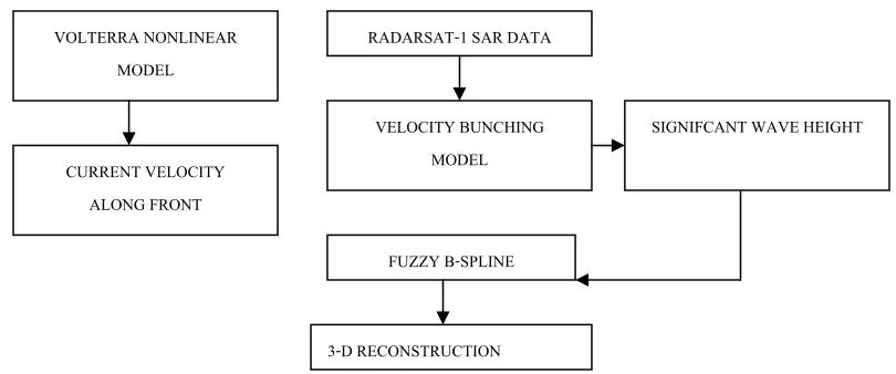
There are three models involved for 3-D front reconstruction; velocity bunching, Volterra and Fuzzy B-spline. Significant wave heights are simulated from RADARSAT-1 SAR image by using velocity bunching model. Fuzzy B-spline used significant wave height information to reconstruct 3-D front. Moreover, front flow pattern is modeled by Volterra model (Figure 1).
Figure 1 Block Diagram for RADARSAT-1 SAR data Processing
2.3 Velocity Bunching Model
In this study, two dimension Fourier Transform ( 2-DFFT) has been applied to a single SAR image frame comprising of 512 x 512 image pixels which was extracted from RADARSAT-1SAR image. The Gaussian algorithm was applied to remove the noise from the image and smoothen the wave spectra into normal distribution curve. The band used in this processing was CHH-band. Each pixel represents a 12.5 m x 12.5 m area for
RADARSAT-1SAR image. The entire image frame of RADARSAT-RADARSAT-1SAR image corresponds to a 6.4 km
RADARSAT-1 SAR DATA
VELOCITY BUNCHING MODEL
FUZZY B-SPLINE
3-D RECONSTRUCTION VOLTERRA NONLINEAR
MODEL
CURRENT VELOCITY ALONG FRONT
included in a single image frame. It is also small enough to show that the ocean can be reasonably assumed homogeneous within a frame (Maged 2004).
The velocity bunching MTF is the dominant component of the linear MTF for the ocean waves with an azimuth wave number (kx). According to Alpers et al., (1981); Vachon et al.,
(1993, 1994, 1995 and 1997), the velocity bunching can contribute to linear MTF based on the following equation
⎥⎦ ⎤ ⎢⎣
⎡ +
= ω sinθ icosθ
k k V
R
M x
v (1)
where R/V is the scene range to platform velocity ratio, which is 111 s in the case of RADARSAT-1SAR image data, θis RADARSAT-1SAR image incidence angel (350-490) and ω is wave spectra frequency which equals to 2Π/K. To estimate the velocity bunching
spectra Svb(k), we modified the algorithm that was introduced by Krogstad and Schyberg
(1991). The modification is to multiply the velocity bunching MTF (Mv) by
RADARSAT-1SAR image spectra variance of the azimuth shifts. This can be calculated by using the following formula:
] ][ )
( !
) ( [
)
( * 2 2
1
2
0 v
K n
n
n x
vb S k e M
n k I
k
S x ρζζ
ζζ ψ
ψ −
∞
=
∑
= (2)
where Sζζis the SAR spectra variance of the azimuth shifts due to the surface motion,
which was induced by the velocity bunching effect in azimuth direction due to high value of R/V. Furthermore, SAR spectra of ocean wave images have a characteristic of azimuth cutoff and also have an intrinsic azimuth cutoff that in many cases fit very well with actual observation and relates to the cutoff directly to the standard deviation of the azimuth shift , which may be compactly related to fundamental sea state parameters. ρζζ is the variance
of the derivative of displacements along the azimuth direction,I0 is SAR image intensity
and “*n” means (n-1) –fold convolution according to Krogsted and Schyberg ( 1991). Equation 2 Is used to draw the velocity bunching spectra energy contours.
Estimation of Significant Wave Height from Velocity Bunching Spectra based on the azimuth cut-off arising from the velocity-bunching model, equation (2), the azimuth cutoff could be scaled by the standard deviation of the azimuth shift. Vachon et al.,(1993) introduced a relationship between the variance of the derivate of displacement along the azimuth directionρζζ and the standard deviation of the azimuth shift σ which were estimated from the velocity bunching spectra. This relationship was given by
ζζ ρ
σ = Vachon et al., (1993) (3)
The relation between standard deviation of the azimuth shift σ and significant wave height
s
H can be given by
s x
H g k V
R 0.5 0.5 2
) 8 ( ) 2
) ( sin 1 )(
( θ
σ = − (Vachon et al., 1994) (4)
where kxis the azimuth wave number, θ is RADARSAT-1SAR image incident angle, R/V is
the scene range to platform velocity ratio and gis the acceleration due to the gravity. Note
that the mean wave period T0 is equal to 2π( kx g)−0.5. Using equation 6 and equation 4,
the significant wave height Hs can be obtained:
0 2 5 . 0
] /
4 / 1 [ ) ( 6 .
0 T
V R Hs
θ ρζζ +
= (5)
where θis the RADARSAT-1SAR incidence angle and equation 5 Is used to estimate the
significant wave height which is based on the standard deviation of the azimuth shift σ .
2.4 Volterra Model
x a g a g a x g x y y x y u V R K j K u U K c K u j U K c K u x u x c t K u x U k v v H r r r r r r r r r r r r r r ) )( . 10 . 6 . 0 .( ] ) ( 043 . 0 [ ] ) ( [ ) ( 043 . 0 . ) ( . . ) ( 043 . 0 [ . ) , ( 4 2 2 1 0 2 2 1 0 2 0 1 1 − − − − − → + + + ⎥⎦ ⎤ ⎢⎣ ⎡ ∂ ∂ ⎥ ⎦ ⎤ ⎢ ⎣ ⎡ + ∂ ∂ + ∂ ∂ + ∂ ∂ ∂ ∂ = ω ω ω ψ ω (6)
whereU→ is the mean current velocity, urxis the current flow while urais current gradient
along azimuth direction, respectively. ky is the wave number along range direction, Kr is
the spectra wave number, ω0is the angular wave frequency, cg
r is the wave velocity group,
ψ is the wave spectra energy and R/V is the range to platform velocity ratio.
In reference to Ingland and Garello, (1990), the inverse filter G(vx,vy)is used since H1y(vx,vy)
has a zero for (vx,vy)which indicates the mean current velocity should have a constant
offset. The inverse filter G(vx,vy)can be given as
⎪⎩ ⎪ ⎨ ⎧ = − 0 )] , ( [ ) , ( 1 1y x y y x v v H v v
G If
. , 0 ) , ( otherwise v
vx y ≠ (7)
Using equation 6 into 7, range current velocity Uy(0,y) can be estimated by
) , ( . ) , 0
( RADARSAT 1SAR x y
y y I G v v
U = − (8)
where IRADARSAT−1SAR is the frequency domain of Radarsat-1 SAR image acquired by
applying 2-D Fourier transform on RADARSAT-1 SAR image.
2.5 The Fuzzy B-splines Method
Based on significant wave height modeled by using velocity bunching and radar backscatter cross section across front, Fuzzy numbers are generated. In doing so,two basic notions that we combined together: confidence interval and presumption level. A confidence interval is a real values interval which provides the sharpest enclosing range for significant wave height values. An assumption level µ -level is an estimated truth value in the [0,1] interval on our
each one related to a assumption level µ [0,1]. Moreover, the following must hold for
each pair of confidence interval which define a number: '
' hfh
fµ ⇒
µ . Let us consider a function f :h→h, of N fuzzy variables h1,h2,....,hn. Where hn are the global minimum
and maximum values of significant wave heights The construction begins with the same pre-processing aimed at the reduction of measured significant wave height values into a uniformly spaced grid of cells. Then, a membership function is defined for each pixel element which incorporates the degrees of certainty of radar cross backscatter.
3. RESULTS AND DISCUSSION
Figure 2 shows the signature of current boundary which can turn up as a result of brightness frontal curved line. Furthermore, it is clear that the front occurred close to estuary, which is a clear indications of tidal front events. In fact, the interaction of flood tidal current flow from estuary with topography can form a tidal front.
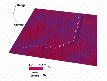
Figure 2 Front signature in RADARSAT-1 SAR and its Backscatter Values
shows that significant wave variation cross front with maximum significant wave height of 1.2 m and gradient current of 0.9 m/s. In fact March represents the northeast monsoon period as coastal water currents in the South China Sea tend to move from the north direction (Maged 1994). Furthermore, Maged (1994) quoted that strong tidal current is a dominant feature in the South China Sea with maximum velocity of 1.5 m/s. The visualization of 3-D front is sharp with the RADARSAT-1 SAR CHH band due to the fact that
each operations on a fuzzy number becomes a sequence of corresponding operations on the respective µandµ'-levels, and the multiple occurrences of the same fuzzy parameters
evaluated as a result of the function on fuzzy variables (Anile 1997). Typically, in computer graphics, two objective quality definitions for Fuzzy B-splines were used: triangle-based criteria and edge-based criteria. Triangle-based criteria follow the rule of maximization or minimization, respectively, the angles of each triangle. The so-called max-min angle criterion prefers short triangles with obtuse angles.
4. CONCLOUSION
This paper demonstrated work done to utilize Fuzzy B-spline to reconstruct ocean surface features such as front by RADARSAT-1 SAR data. Velocity bunching model extracted the elevation of ocean surface which important in building up the topology information requested in Fuzzy B-spline. Front is generated due to tidal current interaction between estuary and ocean. Front is characteristics by 0.9 m/s current flow which concaved along coastal water. In conclusion, Fuzzy B-spline model is considered as good tool to visualize ocean surface feature such as front.
REFERENCES
Alpers, W.R., Ross, D.B. and C.L. Rufenach (1981). On the detectability of ocean surface waves by real and synthetic aperture radar. J. Geophysical Research,
86:6481-6498.
Anile, A. M, (1997) Report on the activity of the fuzzy soft computing group, Technical Report of the Dept. of Mathematics, University of Catania, March 1997, pages 10.
Anile, AM, Deodato, S, Privitera, G, (1995) Implementing fuzzy arithmetic, Fuzzy Sets and Systems, 72.
Inglada, J. and Garello R.,(1999) Depth estimation and 3D topography reconstruction from SAR images showing underwater bottom topography signatures. In Proceedings of IGARSS’99.
Krogstad, H.E., and Schyberg, H. (1991). On Hasselman ’s nonlinear ocean –SAR transformation, Proc. of IGARSS’91, held at Espo, Finland from Jun. 3-6, 1991, pp:841-849.
Maged M, (1994). Coastal Water Circulation off Kuala Terengganu, Malaysia”. MSc. Thesis Universiti Pertanian Malaysia.
Maged M., H. L. Mohd., and K., Yunus. (2002), TOPSAR Model for bathymetry Pattern Detection along coastal waters of Kuala Terengganu, Malaysia. Journal of Physical Sciences. Vol (14)(3), 487-490.
Robinson, I.S. (1994) Satellite Oceanography: An Introduction for Oceanographers and Remote –sensing Scientists. Johan Wiley &Sons. New York.
Shuchman, R.A., Lyzenga, D.R. and Meadows, G.A. (1985)., Synthetic aperture radar imaging of ocean-bottom topography via tidal-current interactions: theory and observations, Int. J. Rem. Sens., 6, 1179-1200.
Simpson, J. H. (1981) The shelf-sea fronts: implications of their existence and behaviour.
Philosophical Transactions of the Royal Society of London A302, 531 - 546.
Simpson, J. H. and R. D. Pingree (1978) Shallow sea fronts produced by tidal stirring. In: M. J. Bowman and W. E. Esaias (editors): Oceanic fronts in coastal processes.
Springer, Berlin, 29 - 42.
Vachon, P.W., Raney,R.K., Krogstad, H.E., and Liu, A.K., (1993). Airborne synthetic aperture radar observations and simulations for waves-in-Ice. J. Geophysical Research, 98:16,411-16,425.
Vachon, P.W., Krogstad, H.E., and Paterson,J.S., (1994). Airborne and spaceborne synthetic aperture radar observations of ocean waves. Atmosphere-Ocean. 32(10): 83-112.
Vachon P.W., Liu, A. K. and Jackson, F.C. (1995). Near-shore wave evolution observed by airborne SAR during SWADE. Atmosphere-Ocean, 2: 363-381.
Vachon, P.W. and Campbell, J.W.M. and Dobson, F.W., (1997). Comparison of ERS and RADARSAT SARS for wind and wave measurement. Paper Presented at third ERS Symp., ESA, held at Florence, Italy from Mar. 18-2, 1997.