Online Sequential Extreme Learning Machine: A New Training Scheme for Restricted Boltzmann Machines

(1)

Page 1 of 7

Online Sequential Extreme Learning Machine: A New

Training Scheme for Restricted Boltzmann Machines

1_{BERGHOUT Tarek}

1_{Laboratory of Automation and Manufacturing Engineering, University of Batna 2, Batna 05000, Algeria;}

[email protected]

Abstract: The main contribution of this paper is to introduce a new iterative training algorithm for restricted

Boltzmann machines. The proposed learning path is inspired from online sequential extreme learning

machine one of extreme learning machine variants which deals with time accumulated sequences of data with

fixed or varied sizes. Recursive least squares rules are integrated for weights adaptation to avoid learning rate

tuning and local minimum issues. The proposed approach is compared to one of the well known training

algorithms for Boltzmann machines named “contrastive divergence”, in term of time, accuracy and

algorithmic complexity under the same conditions. Results strongly encourage the new given rules during

data reconstruction.

Keywords: restricted Boltzmann machine; contrastive divergence; extreme learning machine; online

sequential extreme learning machine; autoencoders; deep belief network; deep learning

1. Introduction

Restricted Boltzmann machine (RBM) is the first types of neural networks used for unsupervised learning.

RBM is a shallow neural network with just two layers, the visible layer and the hidden layer. In RBM network,

each node from the visible layer is connected to every node in the hidden layer. An RBM is considered

restricted because no two nodes in the same layer are sharing connections[1]. In the forward pass, the RBM

iteratively takes a set of inputs and translate them into a set of number that encodes the input. In the

backward pass it takes those set of numbers back to form the reconstructed input. Both forward and backward

movements are known as Gibbs sampling[2].

At the visible layer and after several samplings processes, the reconstructed input is compared to the original

input to determine the quality of the results. A well trained network will be able to perform the backward

translation with a high degree of accuracy. In both steps weights and biases are iteratively tuned to allow the

RBM to decides which features are the most important when detecting patterns[3].

(2)

Page 2 of 7

Generally RBMs are trained using contrastive divergence (CD) algorithm which is often consume more

computational costs due to the need of huge number of hidden nodes[2]. Besides, hyper-parameters such as

learning rate, number of Gibbs sampling, number of hidden neurons and number of iterations vary from an

application to another and needs more human intervention.

In this work and since extreme learning machine (ELM) is widely used for single-batch training in a variety of

application due to its fast training and accuracy [4][5], the contribution of the current experiments is to

introduce a new fast and accurate iterative training algorithm for RBMs by involving ELM theories for both

offline [6]and online learning[7] paradigms. The proposed algorithm experimentally compared to CD

algorithm in term of time and accuracy and the results proves the credibility of the new adopted training

scheme.

This work is organized as follow: in section 1, a brief description about the used training rules of basic online

sequential ELM (OS-ELM) is presented. Section 3 introduces the given rules to the RBM. Section 4, illustrates

with examples the circumstances of the comparative study. Section 5, is the conclusion of this work.

2. Basic OS-ELM

For any given dataset of

n

driven mini-batches of training inputs and targets

{

X T

_k

, }

_k n_k₌₁ where:

1 2 3 ( )

{ ,

,

,....,

}

k i k

X

=

x x x

x

and

T

_k

=

{ , , ,....,

t t t

₁ ₂ ₃

t

_{i k}_{( )}

}

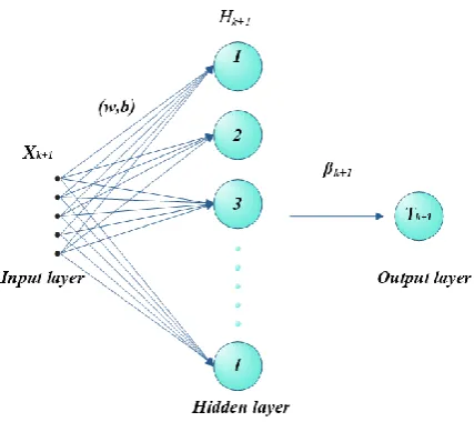
, OS-ELM for a single hidden layer feedforward neural

network (SLFN) has given following training steps in tow different phases[7]:

➢ The initial phase:

• Randomly generated hidden nodes weights and biases

( , )

w b

from any probabilistic distribution.

• Activate the hidden layer

H

of the initial mini-batch using any activation function

G

as addressed in

equation (1).

• Determine the initial output weights



using formula (3) and covariance matrix in formula (2).

➢ The update phase :

• Calculate the hidden layer for any new mini-batch using (1).

• Update the output weights using (4) depending on the prediction error in formula (5), the updated

covariance matrix in formula (6) and the updated gain matrix in formula (7).

1 ( 1 )

k k

H + =G w X + +b (1)

1

0 ( 0 0)

T

(3)

Page 3 of 7 T

0 0 0 0

β = P H T ₍₃₎

T k+1 k k+1 k+1 k+1

β = β - P H e (4)

1 1 1

k k k k

e+ =T+ −H + (5)

1 1 1

T

k k k k k

P₊ =P −K ₊H ₊P ₍₆₎

1

1 1

1

T k

k k

k T

k k

P H K

H P H+ + +

+

= ₍₇₎

The superscripts

( )

−1 and

( )

T

refers to the Moore-Penrose pseudo-inverse of a matrix and the transpose of the

matrix respectively.

Figure 1 addresses the architecture of a SLFN based on the new notations of OS-ELM.

Figure: 1. Architecture of SLFN based OS-ELM.

3. Proposed approach

In the new given rules of RBM the visible layer is mapped using random parameters generated independently

from the training data. The input weights will be tuned each time in a single Gibbs sampling using Sherman

(4)

Page 4 of 7

For the same unlabeled data:

{ ,

1 2

,

3

,....,

( )

}

1

n

k i k k

X

=

x x x

x

₌ , the RBM can be trained also in two distinctive

phases, the initial phase and sequential phase. In the initial phase, the RBM is initialized the same as basic

OS-ELM. The difference between basic OS-ELM and the RBM is that the same input weights are the ones whose

must be updated during the sequential phase. So, equations (4) and (5) must be changed to (8) and (9) to fit the

unsupervised training paradigm.

1 1 1 1

T k k k k k

w₊ =w −P₊ H ₊e ₊ (8)

1

( )

1 1 1

T

T w

k k k k

e

₊

=

X

₊

−

H

₊ − (9)

Unlike old training rules of RBM which use the input weights for reconstruction and their transpose for

reconstruction as shown in equation (10)[8], the new given rules for RBM uses the same tuned weight for

extraction and their transpose of pseudo inverse for feature reconstruction as shown previously in equation

(9). And since the updated weights are determined after activating the hidden layer, there is no need to use

the activation function again. In fact we can map the visible layer directly with the new weights as

demonstrated in (11). Formula (8) is already used for online training of the ordinary autoencoder with ELM

and proved its accuracy and the algorithm is publically available in[9]. Besides, ELM theories allow only the

activation of hidden layer, not the input or the output ones[10].

(

)

(

T

)

H

=

G wX

+

b



X

=

G Hw

+

b

(10)

1

(

T

)

H

=

Xw



X

=

H w

− (11)

Figure 2 addresses the architecture of the proposed RBM with the new notations.

Figure: 2. Architecture of the RBM.

(5)

Page 5 of 7

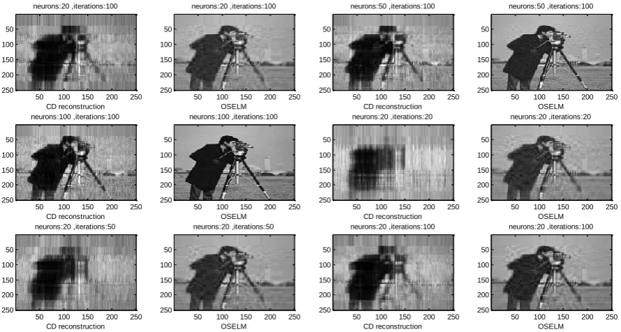
In the current study, the proposed algorithms is compared to CD algorithm during training using the

gray-scaled image of ‘Cameraman’, normalized between 0 and 1 and resized to 250 by 250 pixels. The training

hyper-parameters are adjusted according to Table 1.

Table 1 Training hyper parameters

Methods Gibbs sampling Mini-batch size

CD 5 10

OS-ELM 1 entire data

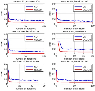
Root mean squared error (RMSE) of reconstruction and training time are the essential evaluation parameters.

Figure 3 shows the reconstruction accuracy according to the number of iteration for different sizes of the

hidden layer.

0 50 100

0 0.2 0.4 0.6 0.8

number of iterations

rm

se

neurons:20 ,iterations:100

CD OSELM

0 50 100

0 0.2 0.4 0.6 0.8

rm

se

CD OSELM

0 50 100

0 0.2 0.4 0.6 0.8

rm

se

CD OSELM

0 5 10 15 20

0 0.2 0.4 0.6 0.8

rm

se

CD OSELM

0 20 40 60

0 0.2 0.4 0.6 0.8

rm

se

CD OSELM

0 50 100

0 0.2 0.4 0.6 0.8

rm

se

CD OSELM

Figure: 3. RMSE behaviour during iterative training.

The new training rules clearly enhance tuning paradigms of the RBM by always outperforming the CD

(6)

Page 6 of 7

towards stopping criteria in less than five iterations, unlike CD which keeps going towards a deeper end and

obviously it needs more than 100 iterations.

By reducing hyper-parameters number and simplifying the Gibbs sampling, computational time will be

gained during training same as Figure 4 explains.

0 20 40 60 80 100 120

0 1 2 3 4 5 6 7 8 9 10 iterations tr a in in g t im e ,s iterations:101 CD OSELM

Figure: 4. Time consuming results during training.

Figure 5 also illustrates and confirms the credibility of the new method compared to CD algorithm.

CD reconstruction neurons:20 ,iterations:100

50 100 150 200 250 50 100 150 200 250 OSELM neurons:20 ,iterations:100

50 100 150 200 250 50 100 150 200 250 CD reconstruction neurons:50 ,iterations:100

50 100 150 200 250 50

100

150 200 250

Figure: 5. Results of image reconstruction using both CD and OS-ELM.

(7)

Page 7 of 7

Comparing to old iterative training algorithms such as contrastive divergence or backpropagation, a new fast

and more accurate training algorithm for RBMs is represented in this work. The new given rules which are

inspired from OS-ELM one of ELM variants allow computational costs reduction under less human

intervention during training.

In the current study the proposed approach is evaluated under unsupervised learning paradigms. Therefore,

the aim of future works will focus on studying the effect of OS-ELM during the training of deep belief neural

networks for supervised learning using a stack of the new RBMs.

References

[1] G. Hafeez et al., “A Novel Accurate and Fast Converging Deep Learning-Based Model for Electrical

Energy Consumption Forecasting in a Smart Grid †,”, energies, 2020.

[2] G. E. Hinton, “A practical guide to training restricted boltzmann machines,” Lect. Notes Comput. Sci. (including Subser. Lect. Notes Artif. Intell. Lect. Notes Bioinformatics), vol. 7700 LECTU, pp. 599–619, 2012.

[3] S. Oh, “Entropy , Free Energy , and Work of Restricted Boltzmann Machines,” ,Entropy, pp. 1–14, 2020. [4] G. Bin Huang, “What are Extreme Learning Machines? Filling the Gap Between Frank Rosenblatt’s

Dream and John von Neumann’s Puzzle,” Cognit. Comput., vol. 7, no. 3, pp. 263–278, 2015.

[5] G. Bin Huang, “An Insight into Extreme Learning Machines: Random Neurons, Random Features and Kernels,” Cognit. Comput., vol. 6, no. 3, pp. 376–390, 2014.

[6] G. Bin Huang, Q. Y. Zhu, and C. K. Siew, “Extreme learning machine: A new learning scheme of

feedforward neural networks,” IEEE Int. Conf. Neural Networks - Conf. Proc., vol. 2, no. August, pp. 985–

990, 2004.

[7] G. Huang, N. Liang, H. Rong, P. Saratchandran, and N. Sundararajan, “On-Line Sequential Extreme

Learning Machine Review of Extreme Learning Ma- chine ( ELM ),” Int. Conf. Comput. Intell., no. Ci, 2005.

[8] Hongming Zhou, Guang-Bin Huang, Zhiping Lin, Han Wang, and Yeng Chai Soh, “Stacked Extreme

Learning Machines,” IEEE Trans. Cybern., vol. 45, no. 9, pp. 2013–2025, 2015.

[9] B. Tarek, “Autoencoders,” 2019. [Online]. Available: BERGHOUT Tarek (2019). Autoencoders

(https://www.mathworks.com/matlabcentral/fileexchange/66080-autoencoders), MATLAB Central File

Exchange. Retrieved October 21, 2019.

[10] G. Bin Huang and L. Chen, “Convex incremental extreme learning machine,” Neurocomputing, vol. 70,